1.1 Introduction

R is a free and open-source interpreted computer programming language runs on Linux, Windows, and macOS. It is modeled after S and S-Plus. The S language was developed in the late 1980s at AT & T labs. The R project was started by Robert Gentleman and Ross Ihaka at the Statistics Department of the University of Auckland in 1995¹. It is now a collaborative project with many contributors and is maintained by the R core-development team.

1.1.1 Installation and setup

You can download R via web browser as well as command line. Choose a installation at your convenience.

1.1.1.1 From Web

Go to CRAN, the Comprehensive R Archive Network, composed of a set of mirror servers distributed around the world and is used to distribute R and R packages. You can try and pick a mirror that’s close to you but try not to! Instead use the cloud mirror, https://cloud.r-project.org, which automatically figures it out for you. Pick the binary as per your OS.

1.1.1.2 From Command line

Linux:
- sudo apt-get install r-base (for Debian and Ubuntu distros)
- sudo pacman -Syu r-base (for Arch distros)
- sudo dnf module install r-base (for CentOS, Fedora and Red Hat Enterprise distros)
- sudo pkg install r-base (for FreeBSD disros)
Windows: winget install -e --id RProject.R
macOS: brew install --cask r

Windows Troubleshooting

For Windows users, you must have to make sure the R executables’ binary folder is added in the system variables path! To check wheather it is there or not, run R (might not work in powershell) or R.exe in your powershell or command prompt. If you notice that R terminal is opened in the command line, you are good to go!

Rterm in Powershell

If R terminal is not opening, follow the instructions:

Go to This PC > Right click on a free space > Properties > Advanced system settings > Environment Variables > Under System Variables click on Path and edit > Add C:\Program Files\R\R-<YOUR_R_VERSION>\bin as a new path

Some Reamrks

A new major version of R comes out once a year, and there are 2-3 minor releases each year. It’s a good idea to update regularly. Upgrading can be a bit of a hassle, especially for major versions, which require you to reinstall all your packages, but putting it off only makes it worse.

1.1.1.3 RStudio

RStudio is an IDE (integrated development environment) exclusively for R programming. Download and install it from here. RStudio is updated a couple of times a year. When a new version is available, RStudio will let you know. It’s a good idea to upgrade regularly so you can take advantage of the latest features.

RStudio Screenshot

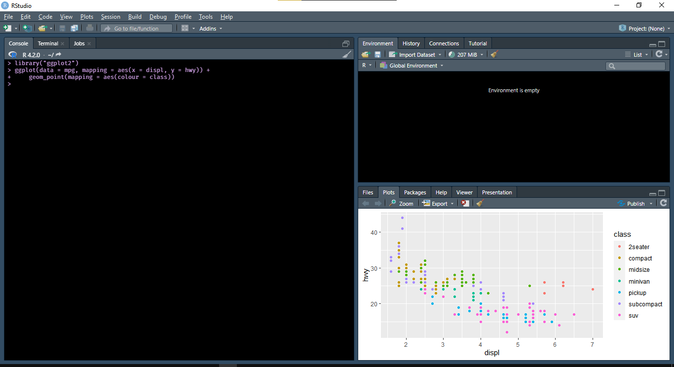
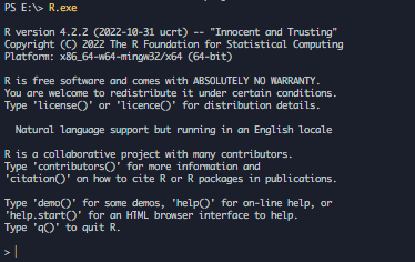
The > represents a prompt indicating that R is waiting for input. At the beginning you just need to know typing and running (press Enter) R code in the console pane. You will learn more stuffs as you go along!

1.1.1.4 R Packages

Sometimes you may need to install some additional packages. An R package is a collection of functions, datasets, documentation that extends the capabilities of base-R. Using packages you can enhance your data exploration capabilities with R.

Before installing a package, first make yourself familiar with R console. You have several options to interact with R but the primary way is command line a.k.a. the console. It is common to all interactive interfaces of R. R commands or statements are executed in R console.

To install a package called UsingR, open RStudio’s R console or native R console (type R in your Shell). Copy the following command in the console and execute (press Enter).

install.packages("UsingR")

Once installed you can add them in the current workspace using the library() function

library("UsingR")

1.1.1.5 VSCode

Microsoft Visual Studio Code is among the most powerful and modern IDEs with productive features and rich support of extensions that makes it one for all, you can work on whatever environment you want! For R, VSCode setup is bit lengthy.

Install the R packages: languageserver, jsonlite and httpgd.

install.packages(
  c("languageserver", "jsonlite", "httpgd"),
  dependencies = TRUE
)

Make sure you have python3 installed as you need to install the python package radian.

pip install radian

Install the R extension for VSCode.
Create a R file and start coding!

The packages - radian and httpgd are used to to enhance your experience of using R in VSCode.

radian is a modern R console that corrects many limitations of the official R terminal and supports many features such as syntax highlighting and auto-completion (just like RStudio console).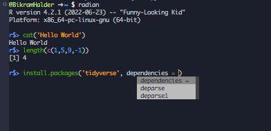
httpgd is an R package to provide a graphics device that asynchronously serves SVG graphics via HTTP and WebSockets. This package is required for the interactive plot viewer of the R extension for VS Code.

VSCode Screenshot

1.1.1.6 Google Colab

Google Colaboratory is a freemium cloud-based tool offered by Google Research that allows users to write and execute Python, Julia and R code in their web browsers. Colab is actually based on the Jupyter open source, and essentially allows you to create and share computation files without having to download or install anything.

Google Colab Screenshot

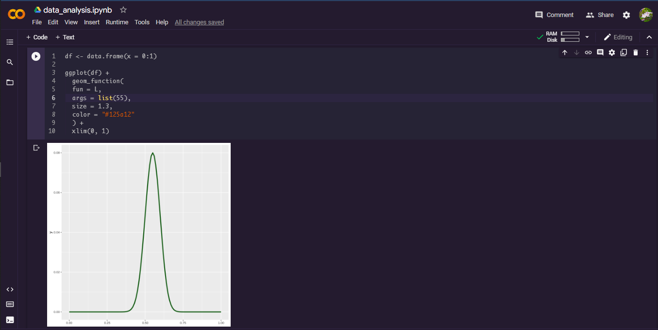
Go to http://colab.to/r or https://colab.research.google.com/notebook#create=true&language=r, to open a google colaboratory in R.

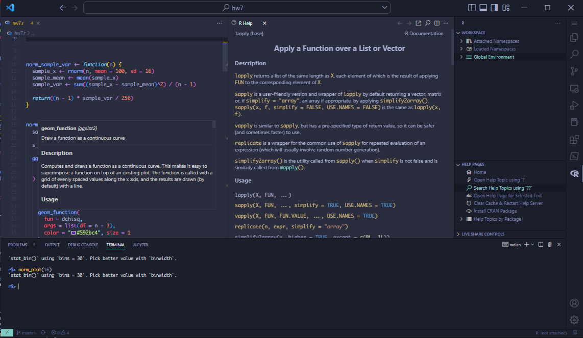
1.1.1.7 R Help

R Help is a great tool to make youself familiar with unknown R stuffs. All the R packages are well documented. You can get information about any function, dataset, package which are currently installed by just executing

?object_name
# or
help(object_name)

Try to get information about max() function for example.

?max
# or
help(max)

It will open a documentation in the bottom right (where you saw the plot) section of RStudio and right half of the editor in VSCode.

And to get help for any keyword type ?? followed by that keyword without space and execute

??keyword
# or
help.search(keyword)

It will search throughout the R documentations of the currently installed packages and show all the results related to that keyword.

Apart from the native R help, you can get the same from RDocumentation, rdrr.io and CRAN Manual.

1.1.2 Preliminary Information

So far you have seen some basic setup. Let’s do some coding so that you can make yourself familiar with R.

1.1.2.1 Basic Coding in R

Calculator

R used standard conventions for math operations: +, -, *, / and ^. Parenthesis () in R is used for grouping as is done in math books. So it can be used as a calculator.

# random computation
((1 / sqrt(2)) * sin(pi / 6) + (1 / sqrt(2)) * cos(pi / 6)) * log(0.6 * 0.4)
#> [1] -1.378489

# complex arithmetic
sqrt(-1)
#> Warning in sqrt(-1): NaNs produced
#> [1] NaN
sqrt(-1 + 0i)
#> [1] 0+1i
Mod(exp(1i * pi / 7))
#> [1] 1

Observe that all of the output above are prefixed with [1], which will make sense when you will learn data vector.

Comments and Assignment

As you might have guessed, # is used for comments. Lines starting with # are skipped by interpreter. What about multiline comments (commenting out more than one line by wrapping some symbols around them)? Unfortunately, R doesn’t support multiline comments. But some people use a trick! Convert the lines you want to comment into a string with "" or ''. R’s interpreter simply prints it as it is, but you should keep in mind that it doesn’t get ignored.

In this book we have used #> to distinguish normal comments and code outputs.

## evaluating complicated expression

# assignment
x_1 <- 5

# assignment doesn't print output
y <- x_1^8 + 9 * x_1^2 - 5 + abs(x_1 - 6) * log(x_1)
y
#> [1] 390846.6

= can also be used for assignment but throughout this book we will use R-community preferred one ,i.e., <-. Don’t be lazy and use =, it might cause coufusion later. Use RStudio keyboard shoutcut: Alt + -(yes, the minus sign). To use the same shourtcut in VSCode, see the setup here

Naming

In R, object names must start with a letter. And it can only contain letters, numbers, _ and . .. To make descriptive names of your object, you may need to use the convention of multiple words. Throughout this book, we will use snake_case where lowercase words are seperated with _. You can use other convention also but we recommend the snake case².

we_use_snake_case <- "We use snake_case"
youMightUseCamelCase
some.may.use.periods

Built-in Variables

There are very few built-in variables in R.

pi
#> [1] 3.141593
T
#> [1] TRUE

1.1.2.2 Functions in R

Functions lies in the heart of computations in R. R is consist of numerous inbuilt functions enabling a rich set of actions. Everyday more and more new functions are added to CRAN.

The `c()` function

Suppose we wish to enter scores (out of 50) in Computer Science class of 10 students. The scores are 40, 39, 15, 6, 18, 22, 30, 21, 15, 23.

scores <- c(40, 39, 15, 6, 18, 22, 30, 21, 15, 23)

c() is generic function³ in R which creates a vector or list of values (kind of same as array) with all of it’s arguments coerced to a common type.

As you have seen before, the value of a variable don’t get automatically displayed unless we call it.

scores
#>  [1] 40 39 15  6 18 22 30 21 15 23

Call a function

R functions are called by function name followed by parenthesis surrounding parameters.

function_name(arg_1 = val1, arg_2 = val2, ...)
# or
function_name(val1, val2, ...)

But latter one is risky! You have to know the exact order of the arguments given in the function definition and assign according to that. The former one is recommended in practice. It is better if you are using a function first time. No matter in what order the arguments are defined, the values can be passed more easily properly to the arguments.

Builtin functions

What is the average score of those students? The answer is the usual average of the scores

(40 + 39 + 15 + 6 + 18 + 22 + 30 + 21 + 15 + 23) / 10
#> [1] 22.9

Writing such manaul expression, is lengthy and time wasting. Instead, use the mean() function.

mean(scores)
#> [1] 22.9
sd(scores)
#> [1] 10.75433

sd() computes \(S = \sqrt{\frac{n}{n-1}\Var{\bf X}}\)

To compute the \(l_2\) distance between (1,9) and (-2,5) we can use the formulae \(\sqrt{(x_1-y_1)^2 + (x_2-y_2)^2}\) as well as a base-R function dist().

((1 - (-2))^2 + (2 - 5)^2)^0.5
#> [1] 4.242641
dist(
  x = rbind(c(1, 2), c(-2, 5)),
  method = "euclidean"
)
#>          1
#> 2 4.242641

You can take advantage of dist() and compute other kind of distances:"maximum", "manhattan", "binary" or "minkowski". To know more use help: ?dist

Explore a big non-exhaustive list of R functions here.

1.1.2.3 Manipulating vectors

Now we are going to show some useful vector manipulations in R. These will extremely helpful when you will manipulate datsets.

As discussed earlier c() is used to create vector with elements coerced to a same type. Individual elements can be accessed by specifying the index inside [] after the variable.

We did a mistake! Marks of 4^th student in scores should be 16 not 6. How to change it?

scores[4] <- 16
scores
#>  [1] 40 39 15 16 18 22 30 21 15 23

The 4th entry is accessed by scores[4] and using assignment operator the value is changed.

Unlike other programming languages, indexing of elements in vectors, lists, data frames, tibbles and other multi-valued data types in R starts from 1 not 0.

Vector arithmetic

Full marks of the CS exam was 50. Scores are to be weighted to 25.

scores_new <- scores * (25 / 50)
## Every member is multiplied with 0.5
scores_new
#>  [1] 20.0 19.5  7.5  8.0  9.0 11.0 15.0 10.5  7.5 11.5

Arithmetic operations of vectors are done member-by-member.

scores_new + scores
#>  [1] 60.0 58.5 22.5 24.0 27.0 33.0 45.0 31.5 22.5 34.5
scores_new - scores
#>  [1] -20.0 -19.5  -7.5  -8.0  -9.0 -11.0 -15.0 -10.5  -7.5 -11.5
scores_new * scores
#>  [1] 800.0 760.5 112.5 128.0 162.0 242.0 450.0 220.5 112.5 264.5
scores_new / scores
#>  [1] 0.5 0.5 0.5 0.5 0.5 0.5 0.5 0.5 0.5 0.5

The same memberwise arithmetic can be done between two vectors.

For unequal length vectors, the shorter one is recycled in order to match the longer vector. It is known as recycling rule.

c(1, 2, 3) + c(10, 2, 90, 8, 6, 3)
#> [1] 11  4 93  9  8  6

Slicing

Can 1^st, 3^rd and 5^th entry be sliced to create a new vector?

score_135 <- scores[c(1, 3, 5)]
score_135
#> [1] 40 15 18

A new vector can be sliced from a given vector with a numeric index vector, consisting of member positions of the original vector to be retrieved. This process is known as slicing of vector.

## Duplicate Indices
scores[c(3, 6, 6)]
#> [1] 15 22 22

## Out-of-order Indices
scores[c(4, 1, 8)]
#> [1] 16 40 21

## Range Index
scores[2:7]
#> [1] 39 15 16 18 22 30

## Removal of elements with specified position vector
scores[-c(1:4)]
#> [1] 18 22 30 21 15 23

Logical operators: `<`, `<=`, `>`, `>=`, `|`, `||`, `&`, `&&` `==` `!`

Which students scored exactly 30?

which(scores == 30)
#> [1] 7

Which students scored less than or equal to 20? How many?

which(scores <= 20)
#> [1] 3 4 5 9
length(which(scores <= 20))
#> [1] 4

Colon operator (`:`)

It is used to generate simple sets of consecutive integers.

vec <- 1:50
vec
#>  [1]  1  2  3  4  5  6  7  8  9 10 11 12 13 14 15 16 17 18 19 20 21 22 23 24 25
#> [26] 26 27 28 29 30 31 32 33 34 35 36 37 38 39 40 41 42 43 44 45 46 47 48 49 50

For a > b, a:b returns a sequence (indeed a vector) from a to b with a step size 1, not exceeding b. In case of a < b, the sequence counts down.

## Can be used to reference all values of a vector
1:length(scores)
#>  [1]  1  2  3  4  5  6  7  8  9 10

## As colon (:) has higer precedence, parentheses are needed
0:(length(vec) - 1)
#>  [1]  0  1  2  3  4  5  6  7  8  9 10 11 12 13 14 15 16 17 18 19 20 21 22 23 24
#> [26] 25 26 27 28 29 30 31 32 33 34 35 36 37 38 39 40 41 42 43 44 45 46 47 48 49
0:length(vec) - 1
#>  [1] -1  0  1  2  3  4  5  6  7  8  9 10 11 12 13 14 15 16 17 18 19 20 21 22 23
#> [26] 24 25 26 27 28 29 30 31 32 33 34 35 36 37 38 39 40 41 42 43 44 45 46 47 48
#> [51] 49

## Slicing the sequence with values less than 10 OR greater than 40
vec[vec < 10 | vec > 40]
#>  [1]  1  2  3  4  5  6  7  8  9 41 42 43 44 45 46 47 48 49 50

Exercises

Exercise 1.1 Hafisa has a log book of time spentby her on Moodle. In the log book she keeps track of the 24-hour reading before each time she logs in. The last 10 readings for a particular student in a day are:

7, 8, 9, 11, 13, 15, 17, 18, 23

Enter these numbers into R as a variable moodle_reading. Use the function diff() on the data. What does it give? Write down, x, the number of hours between each time Hafisa logs into moodle.
Use the max() function to find the maximum number of hours, the mean() function to find the average number of hours and the min() function to get the minimum number of hours for Hafisa between two logins.

Exercise 1.2 Happy Gouda’s quiz scores in Semester II are given below

7, 6, 10, 8, 7, 9, 9, 6, 4, 10, 8, 6, 9, 10

Enter this into R as a variable score_hg. Use the function max() to find the highest score, the function mean to find the average and the function min() to find the minimum.
When confronted by Siva, HG realises that entry 4 was a mistake. It should have been 5. How can you fix this? Do so, and then find the new average.
What does the below command provide in R?
```
sum(score_hg >= 9)
```
What do you get? What percent of your scores are less than 17? How can you answer this with R?

Exercise 1.3 Naina’s cell phone bill varies from month to month. Suppose in her first year of Super DATA (Hons.) program, under the Drop-atmost 10-calls monthly plan, the following monthly amounts were incurred:

460, 330, 390, 370, 460, 300, 480, 320, 490, 350, 300, 480

Enter this data into a variable called naina_bill. Use the sum() function to find the amount spent by Naina that year on the cell phone.
Using R find out what is the smallest amount she spent in a month and the largest amount she spent in a month?
How many months was the amount greater than Rs 400? What percentage was this?
Her monthly loan from NOmoney Bank was Rs 3000. Using R store her balance(after paying her phone bill) in a variable called free_money. Find the average amount available each month for her other expenses.

References

Gregory, Martin, and Merck Serono. 2013. “Generic Functions in R.”

Ihaka, Ross. 2009. “The R Project: A Brief History and Thoughts About the Future.”

White, Homer. 2022. “Beginning Computer Science with R.” In, Generic–Function OO.

Wickham, Hadley. 2019. Style Guide ∙ Advanced R.

Ihaka (2009)↩︎
Wickham (2019)↩︎
White (2022), Gregory and Serono (2013)↩︎