\[ \newcommand{\nRV}[2]{{#1}_1, {#1}_2, \ldots, {#1}_{#2}} \newcommand{\pnRV}[3]{{#1}_1^{#3}, {#1}_2^{#3}, \ldots, {#1}_{#2}^{#3}} \newcommand{\onRV}[2]{{#1}_{(1)} \le {#1}_{(2)} \le \ldots \le {#1}_{(#2)}} \newcommand{\RR}{\mathbb{R}} \newcommand{\Prob}[1]{\mathbb{P}\left({#1}\right)} \newcommand{\PP}{\mathcal{P}} \newcommand{\iidd}{\overset{\mathsf{iid}}{\sim}} \newcommand{\X}{\times} \newcommand{\EE}[1]{\mathbb{E}\left[{#1}\right]} \newcommand{\Var}[1]{\mathsf{Var}\left({#1}\right)} \newcommand{\Ber}[1]{\mathsf{Ber}\left({#1}\right)} \newcommand{\Geom}[1]{\mathsf{Geom}\left({#1}\right)} \newcommand{\Bin}[1]{\mathsf{Bin}\left({#1}\right)} \newcommand{\Poi}[1]{\mathsf{Pois}\left({#1}\right)} \newcommand{\Exp}[1]{\mathsf{Exp}\left({#1}\right)} \newcommand{\SD}[1]{\mathsf{SD}\left({#1}\right)} \newcommand{\sgn}[1]{\mathsf{sgn}} \newcommand{\dd}[1]{\operatorname{d}\!{#1}} \]
1.5 Factors and Levels
In data analysis many times you will deal with categorical data such as Boolean TRUE/FALSE, types of cars, gender, a.k.a., Qualitative variables. They cannot be meaningfully expressed in numbers. But how to handle them in R? The answer is factors and levels. Factors and levels are often useful for Statistical Modeling and Plotting data. Since categorical variables are differnent than continuous variables, storing data as factors ensures that the modeling functions will treat such data correctly9.
In R, A factor is a data structure used to represent a vector as categorical data. You can work with factors and levels in base-R. But some tidyverse packages: dplyr, tidyr, forcats, readr also help to deal with them.
1.5.1 Creating a factor
Using a string to record such variable has two major problems10:
You might make typos
And, the vector doesn’t get sorted in a useful way!
To solve this problem, you need create factor with valid levels.
Get used to
The function factor() is used create a factor. The only required argument to factor() is a vector of values which will be returned as a vector of factor values. Levels are the unique set of values whose order directs the ordering of the factor.
month_levels <- c(
    "January", "February", "March", "April", "May", "June",
    "July", "August", "September", "October", "November", "December"
)
fac_x_month <- factor(x_month, levels = month_levels)
# All the levels are stored with the created factor
fac_x_month
#> [1] June      July      August    September August    July      July
#> [8] August
#> 12 Levels: January February March April May June July August ... December

sort(fac_x_month)
#> [1] June      July      July      July      August    August    August
#> [8] September
#> 12 Levels: January February March April May June July August ... December
And any values not in the set are silently converted to NA.
factor(x_month_2, levels = month_levels)
#> [1] July   August <NA>   <NA>
#> 12 Levels: January February March April May June July August ... December
You can use readr::parse_factor() to get warning.
parse_factor(x_month_2, levels = month_levels)
#> Warning: 2 parsing failures.
#> row col           expected    actual
#>   3  -- value in level set Jamuary
#>   4  -- value in level set Septenber
#> [1] July   August <NA>   <NA>
#> attr(,"problems")
#> # A tibble: 2 × 4
#>     row   col expected           actual
#>   <int> <int> <chr>              <chr>
#> 1     3    NA value in level set Jamuary
#> 2     4    NA value in level set Septenber
#> 12 Levels: January February March April May June July August ... December
By default, levels of any vector are determined by the as.character() function which sorts the values in dictionary order.
Numeric data to factor
Both numeric and character variables can be stored as factors, but levels of a factor are always character values.
x_num <- c(1, 2, 2, 3, 1, 2, 3, 3, 1, 2, 3, 3, 1)
fac_x_num <- factor(x_num)

fac_x_num
#>  [1] 1 2 2 3 1 2 3 3 1 2 3 3 1
#> Levels: 1 2 3
mode(levels(fac_x_num))
#> [1] "character"

mean(x_num)
#> [1] 2.076923

mean(fac_x_num)
#> Warning in mean.default(fac_x_num): argument is not numeric or logical:
#> returning NA
#> [1] NA
fac_x_num is not numeric, so mean(fac_x_num) has returned NA.
To convert fac_x_num into original numeric values, use levels() and as.numeric() functions.
numeric_fac_x_num <- as.numeric(levels(fac_x_num)[fac_x_num])
mode(numeric_fac_x_num)
#> [1] "numeric"
mean(numeric_fac_x_num)
#> [1] 2.076923
You might think the above conversion to numeric vector is equivlent to as.numeric(fac_x_num). But NO! it returns a numeric vector different than the desired11.
1.5.2 Levels and labels in factor
The labels = and levels = arguments in the factor() function are quite confusing. The labels = argument allows you to modify the factor levels names, in other words, it labels the levels. Hence, labels is related to output.
factor(x_month,
    levels = month_levels,
    labels = c(
        "Jan", "Feb", "Mar", "Apr", "May", "Jun",
        "Jul", "Aug", "Sep", "Oct", "Nov", "Dec"
    )
)
#> [1] Jun Jul Aug Sep Aug Jul Jul Aug
#> Levels: Jan Feb Mar Apr May Jun Jul Aug Sep Oct Nov Dec
Whereas, levels is related to input, allowing you to specify how the levels are coded.
Length of labels
labels must have same length as the number of unique groups of the input vector.
gender <- c("male", "female", "female", "male")

# otherwise numbers will be concatinated with it
factor(gender, labels = c("f"))
#> [1] f2 f1 f1 f2
#> Levels: f1 f2

# alphabetical ordering of factors
factor(gender, labels = c("m", "f"))
#> [1] f m m f
#> Levels: m f

# the right way
fac_gender <- factor(gender, levels = c("male", "female"), labels = c("m", "f"))
fac_gender
#> [1] m f f m
#> Levels: m f
The specified labels must have the desired order as levels.
1.5.3 Relevel, Relabel, Reorder
Ordered levels
Even if you ceate a factor with desired levels in order, you won’t be able to do boolean operation on the factor elements.
fac_x_month[1] < fac_x_month[2]
#> Warning in Ops.factor(fac_x_month[1], fac_x_month[2]): '<' not meaningful for
#> factors
#> [1] NA
To fix this issue, you need to set ordered = TRUE which treats the levels as ordered (in the given order).
Relevel
Sometimes you might need to change order of some levels. The relevel() and forcats::fct_relevel() functions can help you12.
relevel(fac_gender, ref = "f")
#> [1] m f f m
#> Levels: f m
fct_relevel(fac_gender, "m", after = 1)
#> [1] m f f m
#> Levels: f m

# Only one level can be put at first
relevel(fac_x_month, "December")
#> [1] June      July      August    September August    July      July
#> [8] August
#> 12 Levels: December January February March April May June July ... November

# forcats::fct_relevel() function extends the capabilities of relevel()
fct_relevel(fac_x_month, "November", "December")
#> [1] June      July      August    September August    July      July
#> [8] August
#> 12 Levels: November December January February March April May June ... OctoberDrop levels
months_random <- factor(x_month,
    levels = c(
        "Garbage", "January", "February",
        "March", "April", "May", "June", "July", "August",
        "September", "October", "November", "December"
    )
)

droplevels(months_random, exclude = "Garbage")
#> [1] June      July      August    September August    July      July
#> [8] August
#> Levels: June July August September
Get info about the levels the in the factor
For a factor, the table() function displays all the levels present in the factor and respective counts.
table(months_random)
#> months_random
#>   Garbage   January  February     March     April       May      June      July
#>         0         0         0         0         0         0         1         3
#>    August September   October  November  December
#>         3         1         0         0         0
When a new factor is created from another factor, it retains only the levels present in the old factor without affecting the order of the levels.
1.5.4 Continuous to Categorical
In data analysis, sometimes it is useful to turn continuous numeric variables into categorical ones. For example, ages of people, exam scores include certain set labels for a certain range of values:
- “baby” for 0-5 years olds, “teen” for 13-19 years olds and so on.
- “A+” for 90-100% marks, “A” for 80-90% marks and blah blah blah.
Using cut()
The cut() function is used to convert a numeric variable into a factor. With breaks = argument, you can specify the number of intervals( \(\geq\) 2) into which the input vector is to be cut.
# 10 iid samples from U(0,1000) distribution
x_unif <- round(1000 * runif(10))

# Breaking into 4 intervals
fac_x <- cut(x_unif, breaks = 4)
fac_x
#>  [1] (550,726] (198,375] (726,903] (550,726] (375,550] (550,726] (375,550]
#>  [8] (198,375] (375,550] (726,903]
#> Levels: (198,375] (375,550] (550,726] (726,903]
table(fac_x)
#> fac_x
#> (198,375] (375,550] (550,726] (726,903]
#>         2         3         3         2

# Labeling the intervals
cut(x_unif, breaks = 3, labels = c("L", "M", "H"))
#>  [1] M L H M M M L L M H
#> Levels: L M H
breaks = also takes a valid numeric vector containing the specified breakpoints.
Break at nice points
The pretty() function yields a nicer set of intervals. It computes a sequence of about \(n+1\) equally spaced rounded numbers covering the range of the values in the input vector. Most of the times the chosen values are 1, 2 or 5 times a power of 10.
xp_factor <- cut(x_unif, breaks = pretty(x_unif, n = 4))
xp_factor
#>  [1] (400,600]   (200,400]   (800,1e+03] (400,600]   (400,600]   (600,800]
#>  [7] (400,600]   (0,200]     (400,600]   (600,800]
#> Levels: (0,200] (200,400] (400,600] (600,800] (800,1e+03]
table(xp_factor)
#> xp_factor
#>     (0,200]   (200,400]   (400,600]   (600,800] (800,1e+03]
#>           1           1           5           2           1
But it may or may not provide the desired levels!
Factor from Quantiles
Quantiles are cut points dividing the observations in a sample into continuous intervals with equal probabilities. You can produce factors based on quantiles of your data to ensure an “equal” distribution.
xq_factor <- cut(x_unif,
    breaks = quantile(x_unif,
        probs = seq(0, 1, by = 0.25)
    )
)
table(xq_factor)
#> xq_factor
#> (199,432] (432,528] (528,628] (628,902]
#>         2         2         2         3
By default, cut() provides half-close intervals as levels. Consequently, it doesn’t include the lowest number! You can fix it by setting include.lowest = TRUE.
xq_factor
#>  [1] (528,628] (199,432] (628,902] (528,628] (432,528] (628,902] (199,432]
#>  [8] <NA>      (432,528] (628,902]
#> Levels: (199,432] (432,528] (528,628] (628,902]

# The fix
xq_factor <- cut(x_unif,
    breaks = quantile(x_unif,
        probs = seq(0, 1, by = 0.25)
    ), include.lowest = TRUE
)
xq_factor
#>  [1] (528,628] [199,432] (628,902] (528,628] (432,528] (628,902] [199,432]
#>  [8] [199,432] (432,528] (628,902]
#> Levels: [199,432] (432,528] (528,628] (628,902]
1.5.5 Date & Time with factors
Converting date and time into factors is often useful for labelling certain period of a year.
First create a date vector of the year 2021
format(), strptime(), strftime() can be used to extract the month from each date using "%b"
month_everyday_2021 <- format(everyday_2021, format = "%b")
head(month_everyday_2021, 3)
#> [1] "Jan" "Jan" "Jan"
df_m_2021 <- as.data.frame(table(month_everyday_2021))

# Changing the names of the variables of the dataframe
names(df_m_2021) <- c("Month", "Freq")
df_m_2021
#>    Month Freq
#> 1    Apr   30
#> 2    Aug   31
#> 3    Dec   31
#> 4    Feb   28
#> 5    Jan   31
#> 6    Jul   31
#> 7    Jun   30
#> 8    Mar   31
#> 9    May   31
#> 10   Nov   30
#> 11   Oct   31
#> 12   Sep   30
You can use unique() function which returns a factor of unique values in the order they are encountered. So the levels argument will provide the month abbreviations in the correct order to produce an properly ordered factor.
# Months as factors
months_2021 <- factor(month_everyday_2021,
    levels = unique(month_everyday_2021),
    ordered = TRUE
)

df_m_2021 <- as.data.frame(table(months_2021))
names(df_m_2021) <- c("Month", "Freq")

df_m_2021
#>    Month Freq
#> 1    Jan   31
#> 2    Feb   28
#> 3    Mar   31
#> 4    Apr   30
#> 5    May   31
#> 6    Jun   30
#> 7    Jul   31
#> 8    Aug   31
#> 9    Sep   30
#> 10   Oct   31
#> 11   Nov   30
#> 12   Dec   31
Let’s see the factored dates by breaking them in week, quarters13
- levels - 53 dates of each week of the year 2021
weeks_2021 <- cut(everyday_2021, breaks = "week")
levels(weeks_2021)
#>  [1] "2020-12-28" "2021-01-04" "2021-01-11" "2021-01-18" "2021-01-25"
#>  [6] "2021-02-01" "2021-02-08" "2021-02-15" "2021-02-22" "2021-03-01"
#> [11] "2021-03-08" "2021-03-15" "2021-03-22" "2021-03-29" "2021-04-05"
#> [16] "2021-04-12" "2021-04-19" "2021-04-26" "2021-05-03" "2021-05-10"
#> [21] "2021-05-17" "2021-05-24" "2021-05-31" "2021-06-07" "2021-06-14"
#> [26] "2021-06-21" "2021-06-28" "2021-07-05" "2021-07-12" "2021-07-19"
#> [31] "2021-07-26" "2021-08-02" "2021-08-09" "2021-08-16" "2021-08-23"
#> [36] "2021-08-30" "2021-09-06" "2021-09-13" "2021-09-20" "2021-09-27"
#> [41] "2021-10-04" "2021-10-11" "2021-10-18" "2021-10-25" "2021-11-01"
#> [46] "2021-11-08" "2021-11-15" "2021-11-22" "2021-11-29" "2021-12-06"
#> [51] "2021-12-13" "2021-12-20" "2021-12-27"- levels - 4 quarters of the year 2021
1.5.6 An Example in Data Visualization: Bar-chart of monthly deceased count
The Master.csv file contains deceased data of COVID-19 patients curated from Government of Karnataka COVID-19 Bulletin. We would like to see a bar chart of monthly deceased count. First load the file:
You can use months() to extract months of reporting date
To plot the data, you need to convert the table into a dataframe.
deceased_df <- as.data.frame(table(deceased_data$month))
names(deceased_df) <- c("month_name", "count")
deceased_df
#> month_name count
#> 1 April 2974
#> 2 August 4108
#> 3 December 430
#> 4 February 483
#> 5 January 843
#> 6 July 3561
#> 7 June 6049
#> 8 March 239
#> 9 May 13599
#> 10 November 737
#> 11 October 2593
#> 12 September 3643
# Plotting
ggplot(data = deceased_df, aes(x = month_name, y = count, fill = month_name)) +
geom_bar(stat = "identity", alpha = .6, width = .4) +
coord_flip() +
scale_fill_viridis_d() +
xlab("") +
theme_bw() But the months doesn’t seem to be in order.
 ggplot() uses ordering alphabetically and treats Month as factor and default level ordering.
Let’s try different approach. Try to arrange the dataframe in a preferred ordering.
deceased_df <- arrange(deceased_df, count)
ggplot(data = deceased_df, aes(x = month_name, y = count, fill = month_name)) +
geom_bar(stat = "identity", alpha = .6, width = .4) +
scale_fill_viridis_d() +
coord_flip() +
xlab("") +
theme_bw()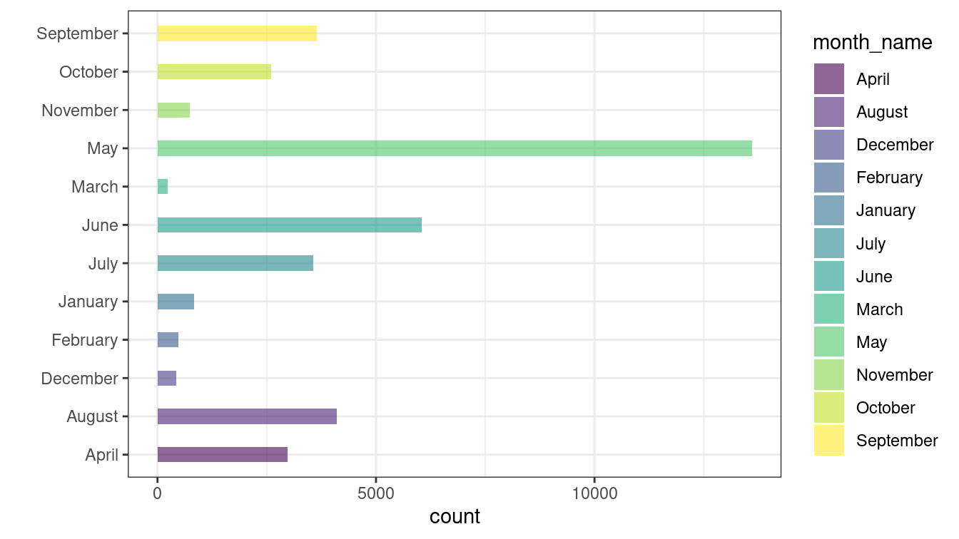 The plot is still the same as before.
 ggplot() takes ordering into account from the factor given by its levels & NOT as we see in the dataframe!
Ah! Factors can solve this problem. Reorder the levels with month_levels.
deceased_df$month_name <- factor(deceased_df$month_name, levels = month_levels)
ggplot(data = deceased_df, aes(x = month_name, y = count, fill = month_name)) +
geom_bar(stat = "identity", alpha = .6, width = .4) +
coord_flip() +
scale_fill_viridis_d() +
xlab("") +
theme_bw()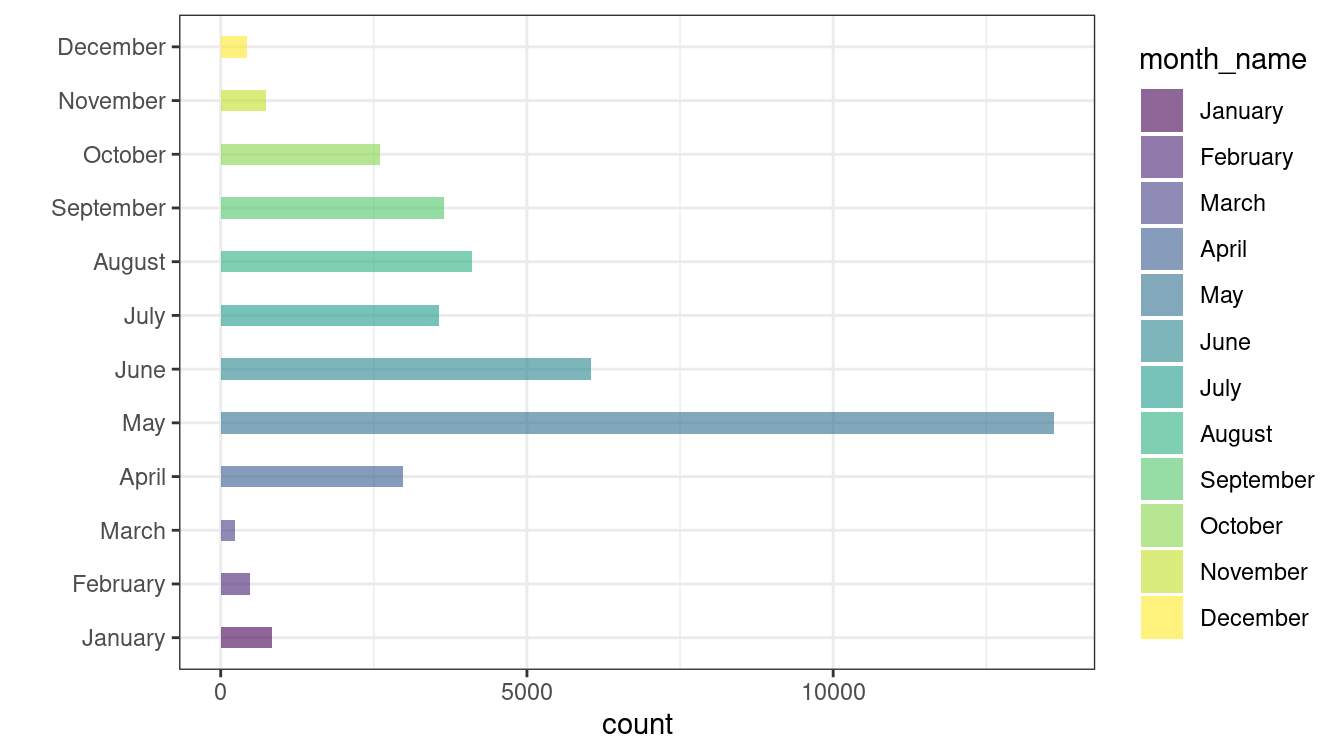 Hurray!
 ggplot() obliges the order now. We get our desired plot.
Some more
You can use forcats::fct_infreq() function to get months according to the order of count.
deceased_data <- read.csv(
    file = "../../assets/datasets/Master.csv",
    header = TRUE
)
deceased_data$month <- months(as.Date(deceased_data$MB.Date))
# Plot
ggplot(
data = deceased_data,
mapping = aes(
x = fct_infreq(month),
fill = cut(Age.In.Years, pretty(Age.In.Years, 4))
)
) +
geom_bar(stat = "count", alpha = .6, width = .4) +
scale_fill_viridis_d() +
xlab("") +
coord_flip() +
theme_bw()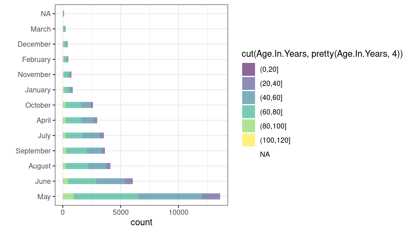 Some more customization to get a nicer plot
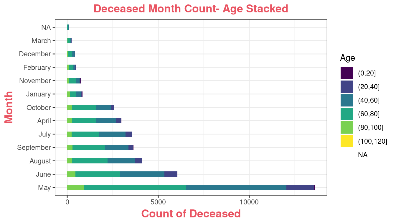
ggplot(
    data = deceased_data,
    mapping = aes(
        x = fct_infreq(month),
        fill = cut(Age.In.Years, pretty(Age.In.Years, 4))
        # cut() is used to add Age.In.Years bin layer
    )
) +
    geom_bar(stat = "count", width = .4) +
    labs(fill = "Age") +
    scale_fill_viridis_d() +
    coord_flip() +
    ggtitle("Deceased Month Count- Age Stacked") +
    ylab("Count of Deceased") +
    xlab("Month") +
    theme_bw() +
    theme(
        plot.title = element_text(
            color = "#e95462",
            size = 14,
            face = "bold",
            hjust = 0.5
        ),
        axis.title.x = element_text(
            color = "#e95462",
            size = 14, vjust = 0.5, face = "bold"
        ),
        axis.title.y = element_text(
            color = "#e95462",
            size = 14, face = "bold"
        )
    )
Exercise
Exercise 1.17 (Function definition syntax in R)
Write functions using the above syantax in R that do each the following: [Decide appropriately what the input and outputs should be. Each item must be separate function that can be called.]
- Find the levels of factor of a given vector.
- Change the first level of a factor with another level of a given factor.
- Create an ordered factor from data consisting of the names of months.
- Concatenate two given factors in a single factor.
- Convert a given vector of integers to an ordered factor.
- Extract the five of the levels of factor created from a random sample from the LETTERS.
- Create a factor corresponding to height in
womendata set, which contains height and weights for a sample ofwomen.