3.5 Confidence Intervals

Suppose you want to estimate a parameter from a distribution \(X\). As you have seen you sample \(X_1, X_2, \dots, X_n\) \(\rm iid\) with \(X\) from the population and construct a estimator function \(g\) and take \(g({\bf X})\) as an estimate of \(\theta\). \(g\) is called

unbiased if \(\EE{g({\bf X})} = \theta\)
consistent if \(\lim_{n \to \infty} \Var{g({\bf X})} = 0\).

As you have seen in the Example 3.2 the Sample mean of an \(\rm iid\) population is an unbiased and consistent estimator of the mean.

Now the question comes,

Can we understand “\(g({\bf X}) - \theta\)” better?
Can you resolve this for \(g({\bf X}) := \overline{X}_n\) using CLT.

Let’s look at it for standard Normal random variable (\(Z \sim N(0,1)\)) We can approximate \[\begin{equation} \tag{3.12} \Prob{\left| Z \right| \leq 1.96} \approx 0.95 \end{equation}\]

2 * (pnorm(q = 0, lower.tail = TRUE) - pnorm(q = -1.96, lower.tail = TRUE))
#> [1] 0.9500042

3.5.1 Getting the intuition

Central limit theorem tells us for \(X_1, X_2, \dots, X_n\) \(\rm iid\) sample from \(X\) with \(\EE{X} = \mu\) and \(\Var{X} = \sigma^2\) \[\begin{equation} \tag{3.13} \Prob{\sqrt{n}\left( \frac{\overline{X}_n - \mu}{\sigma} \right) \leq x} \approx \Prob{Z \geq x} \end{equation}\] for large \(n\).

From, Equation (3.12) and (3.13) we can deduce that, \[\begin{equation} \tag{3.14} \Prob{\left| \sqrt{n}\left( \frac{\overline{X}_n - \mu}{\sigma} \right) \right| \leq 1.96} \approx 0.95 \end{equation}\]

Now, (3.14) is equivalent to (for large \(n\)) \[\begin{align} \Prob{ -1.96\frac{\sigma}{\sqrt{n}} \leq \overline{X}_n - \mu \leq 1.96\frac{\sigma}{\sqrt{n}} } &\approx 0.95 \nonumber \\ \textsf{i.e., } \Prob{ \overline{X}_n -1.96\frac{\sigma}{\sqrt{n}} \leq \mu \leq \overline{X}_n + 1.96\frac{\sigma}{\sqrt{n}} } &\approx 0.95 \nonumber \\ \textsf{i.e., } \Prob{ \mu \in \left[ \overline{X}_n -1.96\frac{\sigma}{\sqrt{n}}, \overline{X}_n + 1.96\frac{\sigma}{\sqrt{n}} \right] } &\approx 0.95 \tag{3.15} \end{align}\] Denote, \(\textsf{Interval}_n\) (or \(I_n\)) as \(\left[ \overline{X}_n -1.96\frac{\sigma}{\sqrt{n}}, \overline{X}_n + 1.96\frac{\sigma}{\sqrt{n}} \right]\) and \(\textsf{True mean}\) as \(\mu\). So, Equation (3.15) is equivalent to \[\begin{equation} \tag{3.16} \Prob{\textsf{True mean} \in \textsf{Interval}_n} \approx 0.95 \end{equation}\] for large \(n\)

Confidence interval is also a statistical estimate of the paramater of the underlying distribution. As we want to estimate the paramater \(\mu\), instead of \(\overline{X}_n\) (point estimator for \(\mu\)) we can provide a \(95\%-\)confidence interval as an estimate for \(\mu\).

How large should \(n\) be to take the \(\approx\) into effect?
It can be answered with Berry-Eseen bound

Does (3.16) implies that there is \(95\%\) chance that \(\mu \in I_n\)?
A big NO! Be careful in the interpretation of (3.16). Let’s look at an example

Example 3.6 Assume that we have, \(I_{n} = (-3,1)\) from one sample and \(I_{n} = (-5,-4)\) from another sample. Clearly, the interpretation of (3.16) above is not correct!

Interpret it correctly, Do the experiment of sampling \(X_1, X_2, \dots, X_n\) \(\rm iid\) form \(X\) and compute \(I_n = \left[ \overline{X}_n -1.96\frac{\sigma}{\sqrt{n}}, \overline{X}_n + 1.96\frac{\sigma}{\sqrt{n}} \right]\). Repeat it \(100\) times. Let, \(I_n^{(1)}, I_n^{(2)}, \ldots, I_n^{(100)}\) be the intervals computed in each trial. (3.16) implies that the \(\textsf{True mean}, \mu\) will belong to \(95\) of these intervals.

Because, \(n-\)large fixed, set \(A = \left\{ \mu \in \left[ \overline{X}_n -1.96\frac{\sigma}{\sqrt{n}}, \overline{X}_n + 1.96\frac{\sigma}{\sqrt{n}} \right] \right\}\). Then, (3.16) tells that \[\begin{equation*} \Prob{A} = 0.95 \end{equation*}\] That is, if we perform \(m\) trials of the experiment and construct \(I_n^{(1)}, I_n^{(2)}, \ldots, I_n^{(m)}\) then \(A\) will occur approximately \(95\%\) of the time.

3.5.2 Simulation

We can simulate Binomial samples either by rbinom() of replicate() function.

Generating \(100\) \(\Bin{10, 0.1}\) samples

bin_sim_1 <- rbinom(100, 10, 0.1)

\(100\) \(\Bin{10, 0.25}\) samples

bin_sim_2 <- replicate(100, rbinom(1, 10, 0.25))

and \(100\) \(\Bin{10, 0.5}\) samples

bin_sim_3 <- rbinom(100, 10, 0.5)

plt_bin_sim_1 <- function(vec, p, text = "") {
  ggplot() +
    geom_histogram(
      mapping = aes(vec),
      binwidth = 1,
      colour = "#000000",
      fill = "#2cb17e"
    ) +
    xlab(TeX(paste0("${", text, "Bin}(10,", p, ")$"))) +
    ylab("frequency")
}

TeX() function is included from latex2exp package

# left
plt_bin_sim_1(vec = bin_sim_1, p = 0.1)

# middle
plt_bin_sim_1(vec = bin_sim_2, p = 0.25)

# right
plt_bin_sim_1(vec = bin_sim_3, p = 0.5)

Look at the histogram of the 3 simulation

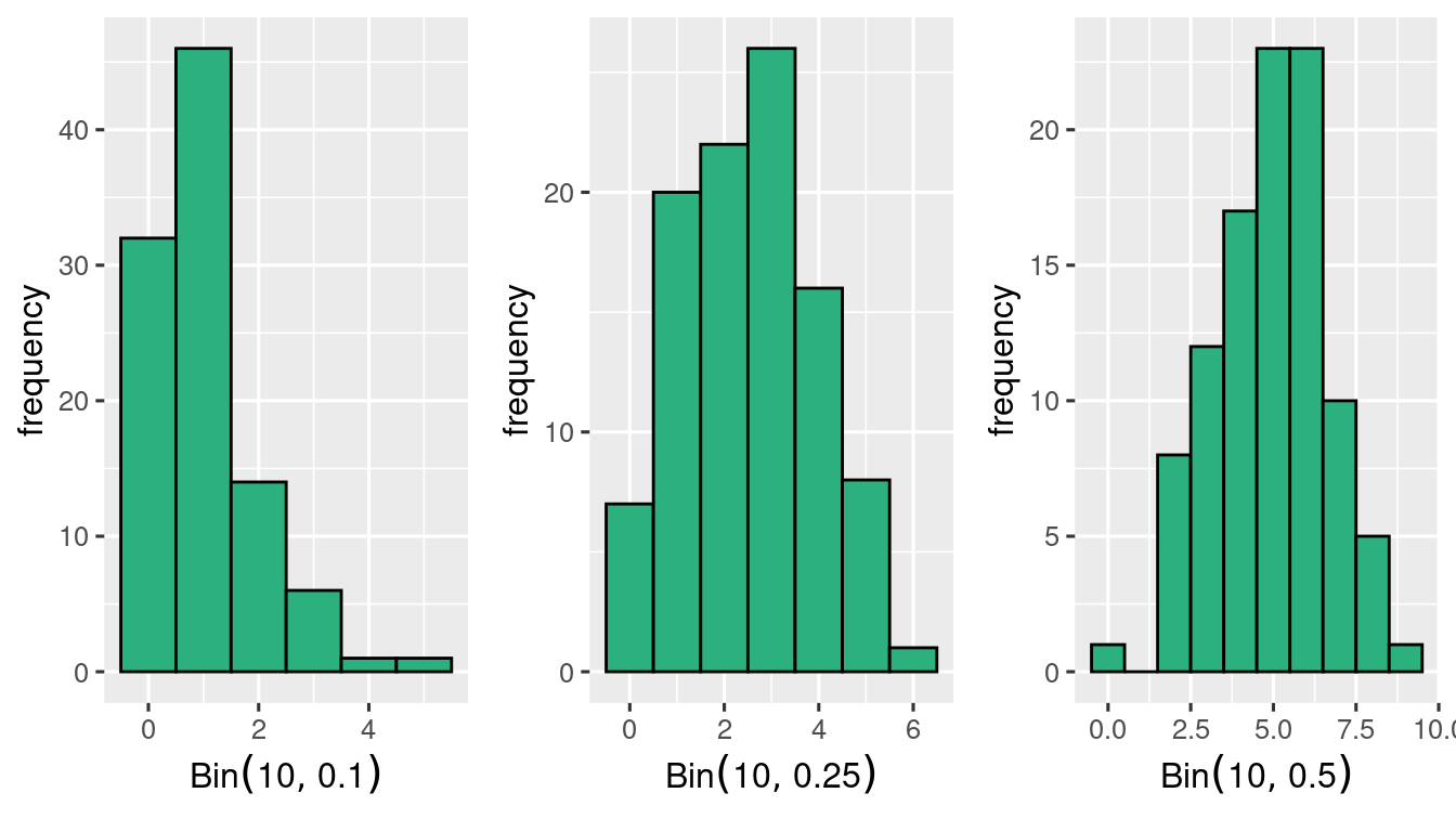
it seems that at \(n=10\) the symmetry is achieved when \(p=0.5\) and not at \(p=0.1\) and \(p=0.25\)
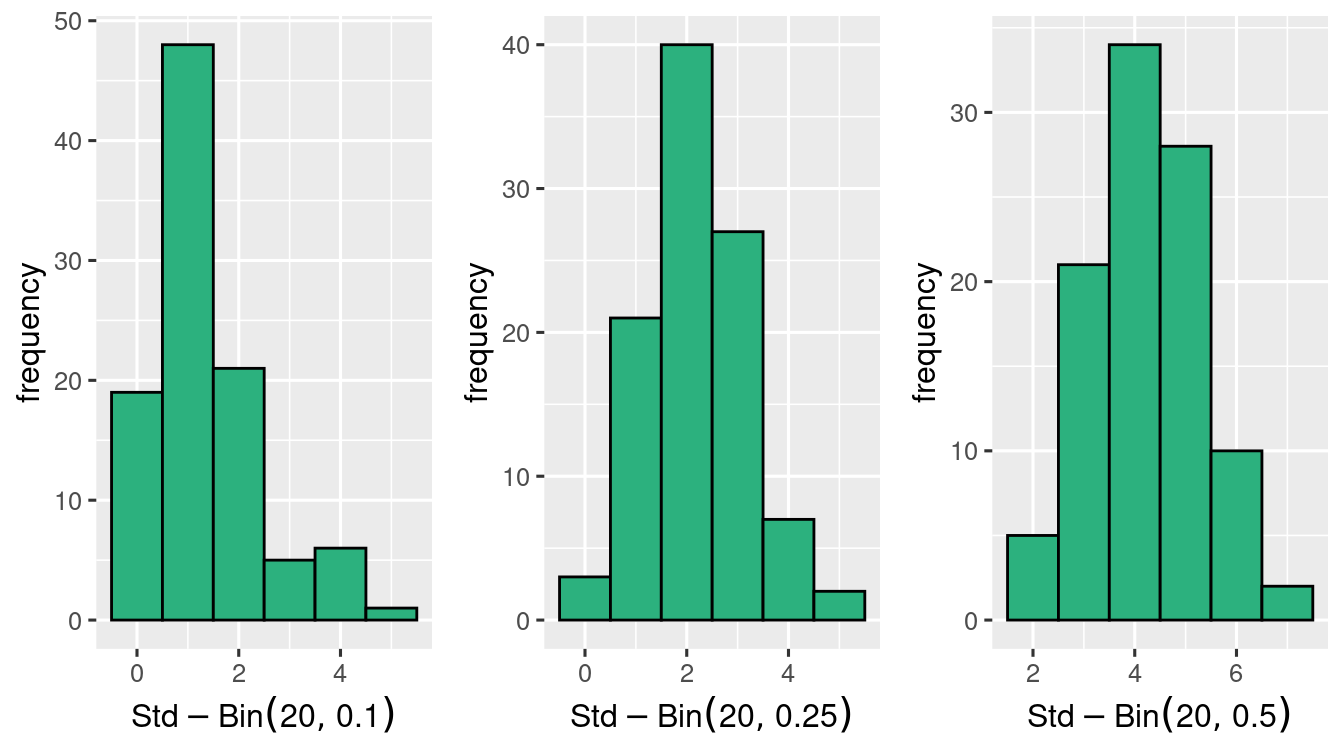
standardisation gives,

with the same \(p\)’s \(n=20\) seems better.

and \(n=50\) gets closer to Normal distribution!

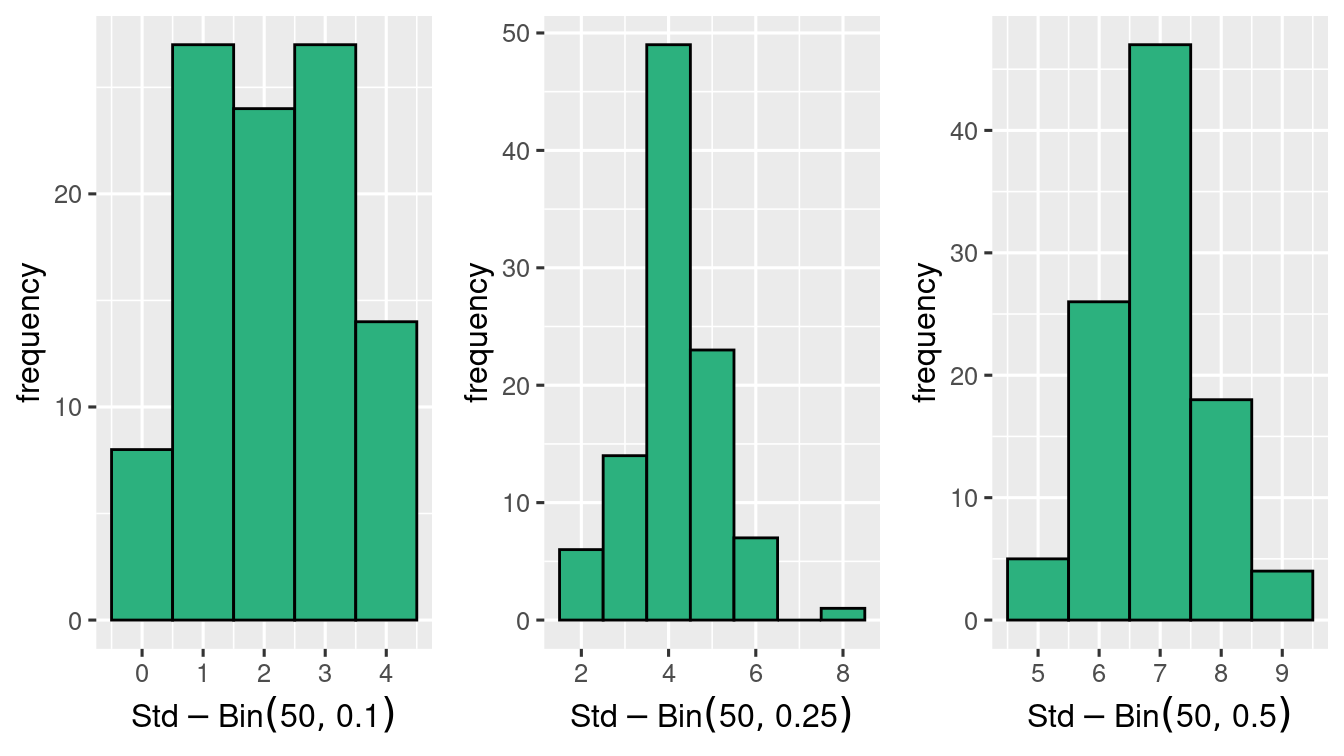
Binomial Random variable is close to Normal when the distribution is symmetric. That is when \(p\) is close to \(0.5\). Otherwise the general rule that we can apply is that when \(np \geq 5\) and \(n(1-p) \geq 5\), then \(\Bin{n,p}\) is close to Normal distribution.

As you have seen earlier, \(95\%-\)confidence interval for \(\mu\) is \(\left[ \overline{X} -1.96\frac{\sigma}{\sqrt{n}}, \overline{X} + 1.96\frac{\sigma}{\sqrt{n}} \right]\) means that,

for \(n\) large if we did \(m\) (large) repeated trials and computed the above interval for each trial then true mean would belong to approximately \(95\%\) of \(m\) intervals calculated.

with this interpretation you can simulate confidance interval for any data. Below, the conf_int() function gives \(100\X\)alpha\(\%-\)confidance interval for a data x

conf_int <- function(x, alpha = 0.95) {
  z <- qnorm(
    (1 - alpha) / 2,
    lower.tail = FALSE
  )
  return(
    c(
      mean(x) - z * sqrt(1 / length(x)),
      mean(x) + z * sqrt(1 / length(x))
    )
  )
}

\(95\%-\)confidence interval for samples \(\pnRV{X}{100}{(1)} \iidd N(0,1)\)

x_1 <- rnorm(100, 0, 1)
y_1 <- conf_int(x = x_1)
y_1
#> [1] -0.2472390  0.1447538

\(95\%-\)confidence interval for samples \(\pnRV{X}{100}{(2)} \iidd N(0,1)\)

x_2 <- rnorm(100, 0, 1)
y_2 <- conf_int(x = x_2)
y_2
#> [1] -0.1126738  0.2793190

\(95\%-\)confidence interval for samples \(\pnRV{X}{100}{(3)} \iidd N(0,1)\)

x_3 <- rnorm(100, 0, 1)
y_3 <- conf_int(x = x_3)
y_3
#> [1] -0.2979872  0.0940056

question comes, “Does \(0\) belong to all the three confidence intervals?”

The below is a plot of the three confidence intervals computed above

par(mfrow = c(1, 3))

plot(c(0, 0), y_1, type = "l", xlab = "", ylab = "", axes = FALSE)
axis(2, at = c(-0.25, -0.15, -0.1, 0, 0.1, 0.15, 0.25))
points(0, 0, pch = 19, col = "blue")
points(0, y_1[1], pch = 23, col = "brown")
points(0, y_1[2], pch = 24, col = "brown")

plot(c(0, 0), y_2, type = "l", xlab = "", ylab = "", axes = FALSE)
axis(2, at = c(-0.25, -0.15, -0.1, 0, 0.1, 0.15, 0.25))
points(0, 0, pch = 19, col = "blue")
points(0, y_2[1], pch = 23, col = "brown")
points(0, y_2[2], pch = 24, col = "brown")

plot(c(0, 0), y_3, type = "l", xlab = "", ylab = "", axes = FALSE)
axis(2, at = c(-0.25, -0.15, -0.1, 0, 0.1, 0.15, 0.25))
points(0, 0, pch = 19, col = "blue")
points(0, y_3[1], pch = 23, col = "brown")
points(0, y_3[2], pch = 24, col = "brown")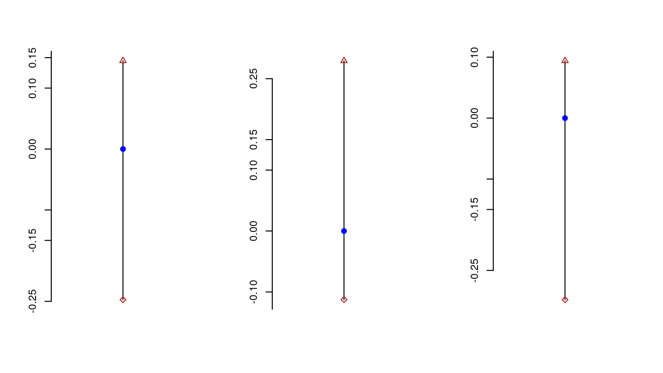

indeed 0 belongs to all the three intervals above!

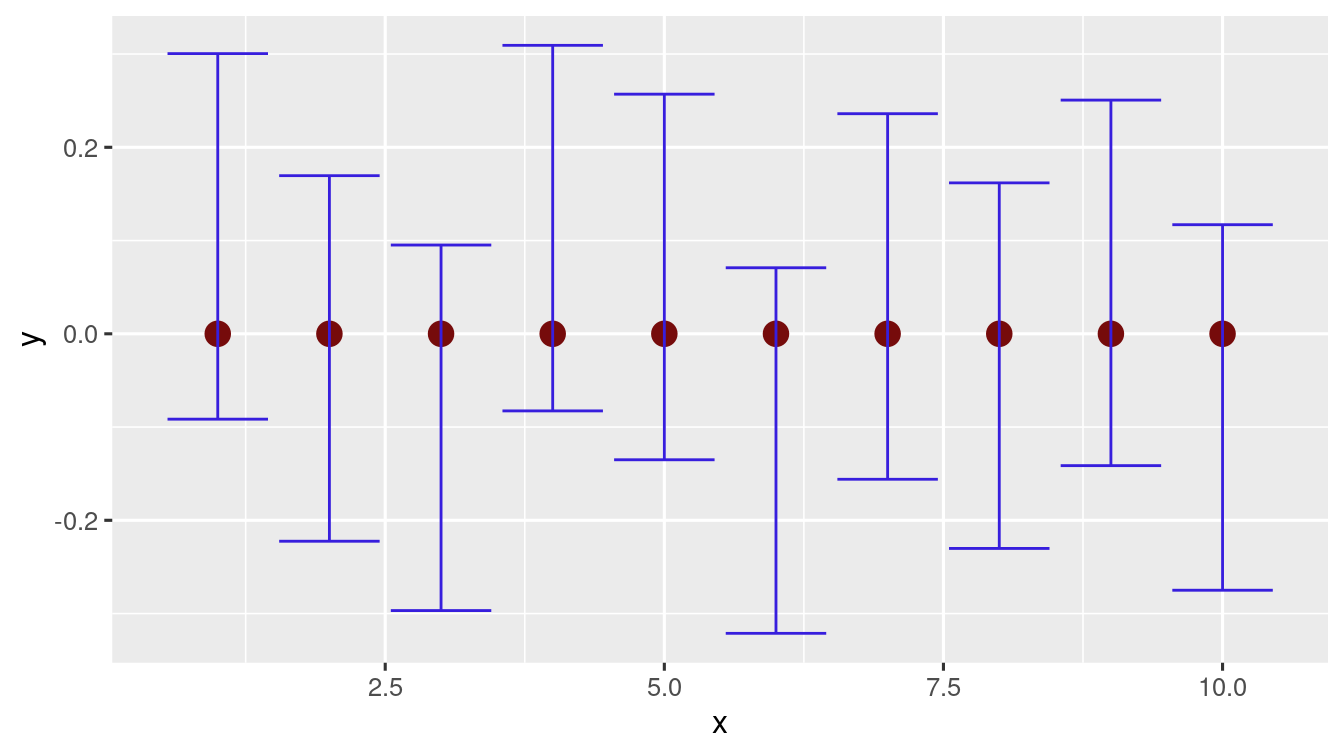
To see in more details, generate \(10\) trials of \(100\) samples from \(N(0,1)\) and compute the confidence intervals using the function defined earlier.

norm_data <- replicate(10, rnorm(100, 0, 1), simplify = FALSE)
norm_ci_data <- sapply(X = norm_data, FUN = conf_int)

Easily you can check how many of them contain \(0\)

table(norm_ci_data[1, ] * norm_ci_data[2, ] < 0)
#> 
#> TRUE 
#>   10

# plotting the above 10 trials
norm_df <- data.frame(
  x = 1:10,
  z_1 = norm_ci_data[1, ],
  z_2 = norm_ci_data[2, ]
)
ggplot(norm_df, aes(x = x, y = 0)) +
  geom_point(size = 4, color = "#760b0b") +
  geom_errorbar(
    aes(ymax = z_2, ymin = z_1),
    color = "#371edd"
  )

\(40\) trials

#> 
#> FALSE  TRUE 
#>     3    37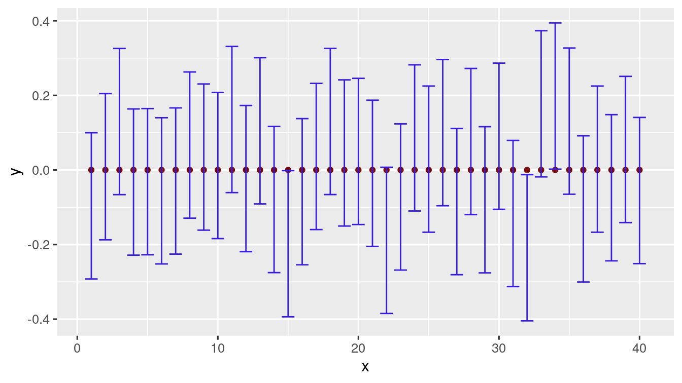

\(100\) trials

#> 
#> FALSE  TRUE 
#>     2    98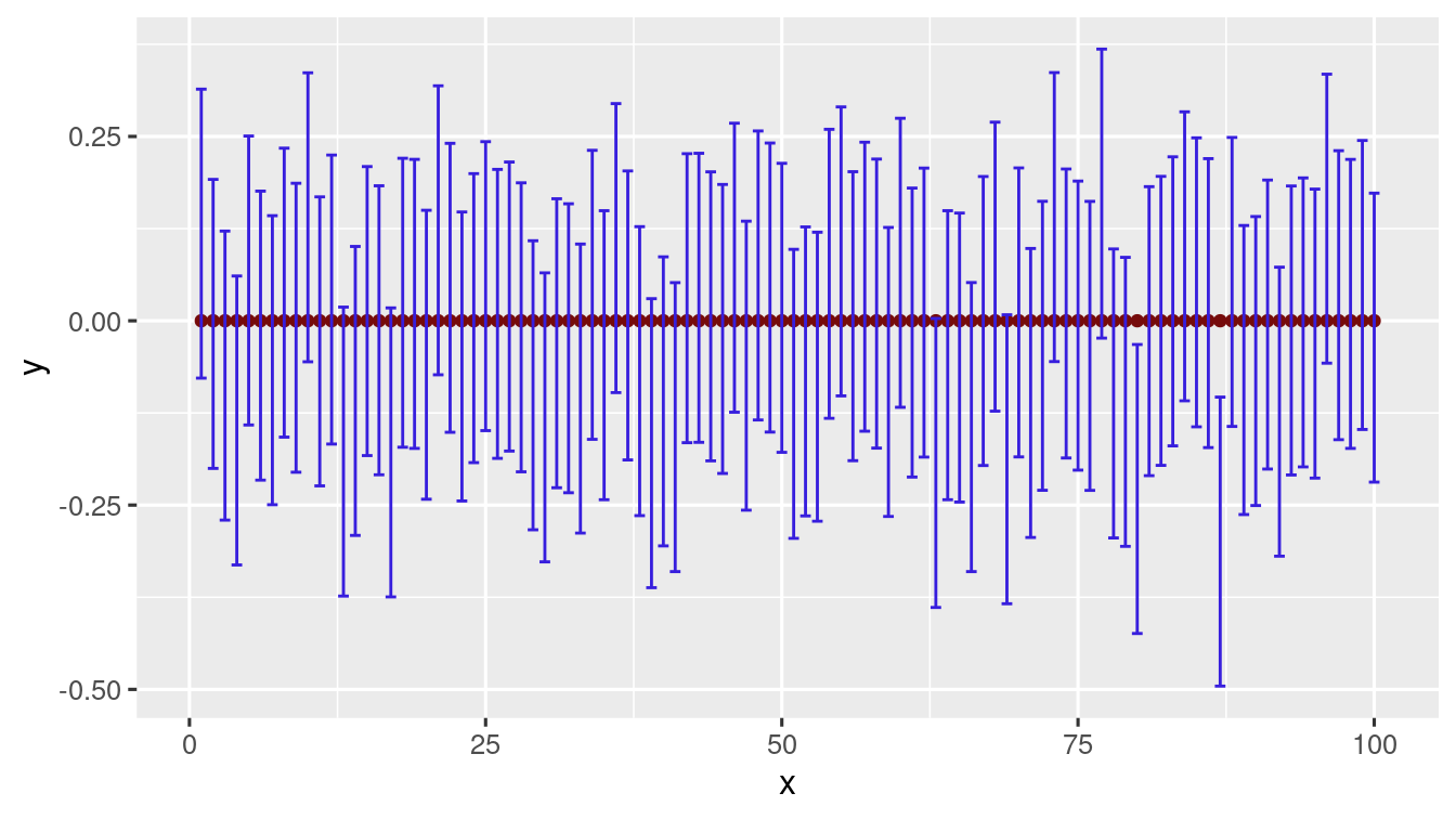

Numerically the interpretation of the confidance interval (as we saw earlier) seems to hold for a Normal population.

Exercises

Exercise 3.11 (Poission Distribution) Consider the \(\Poi{1}\) distribution.

Generate \(100\) trials of \(500\) samples respectively.
Find the \(95\%-\)confidence interval for the mean in each trial.
Compute the number of trials in which the true mean lies in the interval.

Exercise 3.12 The dataset bangalore_rain.data contains \(100\) year monthly rainfall data for Bangalore.

Decide if any month’s \(100\) year rainfall is Normally distributed.
Calculate the yearly total rain fall for each of the \(100\) years.
Plot the histogram and Decide if the distribution is Normal.
Find the \(95\%-\)confidence interval for the expected annual rainfall in Bangalore.

Exercise 3.13 (Normal Distribution) Simulate \(1000\) samples from \(N(0, 1)\) in R. Implement R-codes to do the following:

Assume that variance known to be \(1\). Find a \(95\%-\)confidence interval for the mean \(\mu\).
Assume that variance unknown to be \(1\). Find a \(95\%-\)confidence interval for the mean \(\mu\).

Exercise 3.14 Cracker-Free-rang-dal wants to understand the noise level of firecracker \(10000\) strip. Measuring the noise level of a random sample of \(12\) crackers, it gets the following data (in decibels).

94.0, 98.6, 96.8, 95.5, 93.8, 95.6, 99.3, 95.8, 93.9, 90.2, 91.0, 93.9

Find a \(95\%-\)confidence interval for the average noise level of such crackers. Do not round the final answer. Enter the data with \(1\) decimal place.

Exercise 3.15 Use the inbuilt iris data set in R. For each of the species setosa, versicolor, virginica find a \(95\%-\)confidence interval for: Sepal.Length, Sepal.Width, Petal.Length, and Petal.Width