\[ \newcommand{\nRV}[2]{{#1}_1, {#1}_2, \ldots, {#1}_{#2}} \newcommand{\pnRV}[3]{{#1}_1^{#3}, {#1}_2^{#3}, \ldots, {#1}_{#2}^{#3}} \newcommand{\onRV}[2]{{#1}_{(1)} \le {#1}_{(2)} \le \ldots \le {#1}_{(#2)}} \newcommand{\RR}{\mathbb{R}} \newcommand{\Prob}[1]{\mathbb{P}\left({#1}\right)} \newcommand{\PP}{\mathcal{P}} \newcommand{\iidd}{\overset{\mathsf{iid}}{\sim}} \newcommand{\X}{\times} \newcommand{\EE}[1]{\mathbb{E}\left[{#1}\right]} \newcommand{\Var}[1]{\mathsf{Var}\left({#1}\right)} \newcommand{\Ber}[1]{\mathsf{Ber}\left({#1}\right)} \newcommand{\Geom}[1]{\mathsf{Geom}\left({#1}\right)} \newcommand{\Bin}[1]{\mathsf{Bin}\left({#1}\right)} \newcommand{\Poi}[1]{\mathsf{Pois}\left({#1}\right)} \newcommand{\Exp}[1]{\mathsf{Exp}\left({#1}\right)} \newcommand{\SD}[1]{\mathsf{SD}\left({#1}\right)} \newcommand{\sgn}[1]{\mathsf{sgn}} \newcommand{\dd}[1]{\operatorname{d}\!{#1}} \]

4.4 The \(\chi\)² tests

In the mid-19th century, Gregor Mendel conducted experiments on garden pea plants and formulated the laws of genetics. However, he analyzed the data intuitively, as formal statistical methods were not available at that time. In the 1930s, Ronald Fisher reconstructed Mendel’s experiments and found inconsistencies in the observed data¹⁵. He introduced the \(\chi^2\) test to evaluate the goodness of fit of observed data to expected distributions.

The \(\chi^2\) test helps answer questions like:

1. Are the dice we roll in our experiments fair?
2. Are two populations independent?

To generalize these questions:

1. How well does the distribution of the data fit the model?
2. Does one variable affect the distribution of another?

Specifically we want to understand how “close” the observed values are to the expected values under the fitted model:

1. In the first case, we determine whether the distribution of results in a sample could plausibly come from a specified null hypothesis distribution. This is known as \(\chi\)² test for “goodness of fit”.
2. In the second case, we calculate the test statistic by comparing the observed count of data points within specified categories to the expected number of results in those categories under the null hypothesis. We call it \(\chi\)²\(-\)test of independence.

4.4.1 \(\chi\)² test for “goodness of fit”

We seek to determine whether the distribution of results in a sample could plausibly have come from a distribution specified by a null hypothesis. The test statistic is calculated by comparing the observed count of data points within specified categories relative to the expected number of results in those categories according to the assumed null.

Let \(T\) be a random variable with a finite range \(\{c_1, c_2, \ldots, c_k\}\) and probabilities \(\Prob{T=c_j} = p_j > 0\) for \(1 \leq j \leq k\). Consider a sample \(X_1, X_2, \dots, X_n\) drawn from the distribution of \(T\), let \(Y_j = \left| \{ k \mid X_k=c_j \} \right|\) be the number of sample points with outcome \(c_j\) for \(1 \leq j \leq k\). We perform the test for the following hypothesis:

• Null Hypothesis (\(H_0\)): The distribution comes from a multinomial distribution with parameters \(p_1, p_2, \ldots, p_k\).
• Alternate Hypothesis (\(H_A\)): The distribution comes from a multinomial distribution with at least one parameter different from \(p_1, p_2, \ldots, p_k\).

The \(\chi^2\) test statistic is given by: \[\begin{align*} X^2 & := \sum_{j=1}^k \frac{(Y_j - np_j)^2}{np_j} \\ & \left( \equiv \sum_{j=1}^k \frac{(\textsf{Observed} - \textsf{Expected})^2}{\textsf{Expected}} \right) \end{align*}\]

So, \(X^2\) asymptotically follows a \(\chi^2\) distribution with \(k-1\) degrees of freedom as \(n \to \infty\). Note that the \(np_j\) term is the expected number of observations of the outcome \(c_j\), so the numerator of the fractions in the χ2 computation measures the squared difference between the observed and expected counts.

Choose a significance level \(\alpha\) and use the \(\chi^2\) distribution to compute the \(p-\)value \(\Prob{X^2 \geq \chi^2_{k-1}}\).

A formal proof of the statement above requires a deeper understanding of linear algebra than we assume as a prerequiste for this text, but below we demonstrate its truth in the special case where \(k = 2\) and we provide the formal technical details in the appendix. The approximation itself relies on the Central Limit Theorem and as with that theorem, larger values of \(n\) will tend to lead to a better approximation. Before proceeding to the proof, we present an example will help illustrate the use of the test.

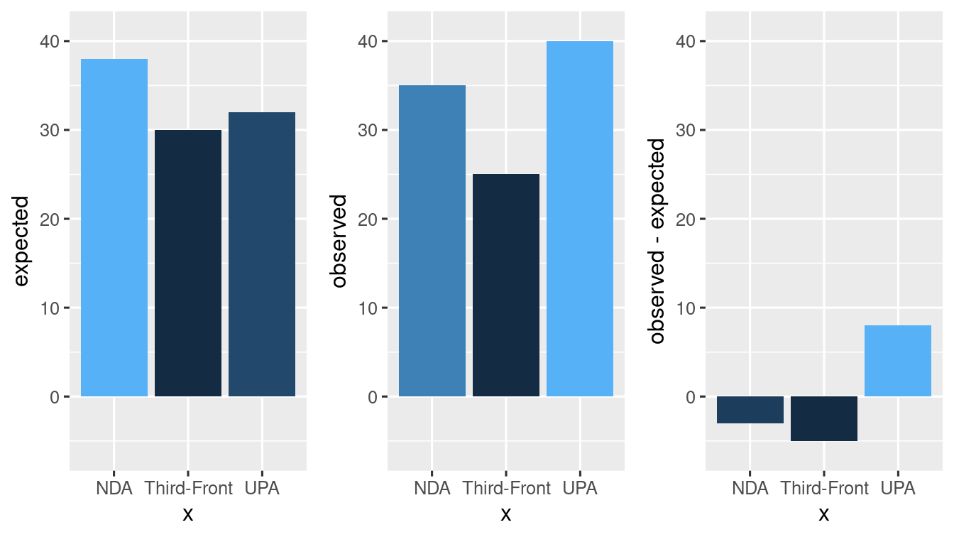
Example 4.4 In a recent election, political parties in India were divided into three major alliances: NDA, UPA, and Third-Front. The previous election results showed support of 38%, 32%, and 30% for these alliances, respectively. To assess whether the vote share has changed, a sample of 100 people was taken by the Super-Nation TV channel. The results of the sample showed 35 in favor of NDA, 40 in favor of UPA, and 25 in favor of Third-Front. The TV channel concludes that the vote share has not changed and tests this hypothesis. Is this a plausible claim given the observed results?

We can compare the observed results to the expected results under the assumption of no change. The expected distribution, based on the previous election percentages, is (38, 32, 30). Subtracting the observed from the expected gives us (35-38, 40-32, 25-30).

# Define the observed data and expected probabilities
observed_data <- c(35, 40, 25)
prob <- c(0.38, 0.32, 0.3)

# Compute the test statistic
n <- 100
test_statistic <- sum((observed_data - n * prob)^2 / (n * prob))

# Compute the p-value
p_value <- pchisq(test_statistic, df = 2, lower.tail = FALSE)

# Create a data frame for visualization
test_df <- data.frame(
  x = c("NDA", "UPA", "Third-Front"),
  observed = observed_data,
  expected = 100 * prob,
  stringsAsFactors = FALSE
)

# Create bar plots for observed, expected, and difference
plt_obs <- test_df |> ggplot() +
  geom_bar(
    mapping = aes(
      x = x, y = observed,
      fill = observed
    ),
    stat = "identity"
  ) +
  theme(legend.position = "none") +
  ylim(-6, 41)

plt_exp <- test_df |> ggplot() +
  geom_bar(
    mapping = aes(
      x = x, y = expected,
      fill = expected
    ),
    stat = "identity"
  ) +
  theme(legend.position = "none") +
  ylim(-6, 41)

plt_diff <- test_df |> ggplot() +
  geom_bar(
    mapping = aes(
      x = x, y = observed - expected,
      fill = observed - expected
    ),
    stat = "identity"
  ) +
  theme(legend.position = "none") +
  ylim(-6, 41)

The resulting \(p-\)value from the chi-square test is 0.2154368. By comparing this \(p-\)value to a chosen significance level (e.g., 0.05), we can determine whether to reject the hypothesis of no change in the vote share.

4.4.2 \(\chi\)²\(-\)test of independence

A common way to present Bivariate data is through a contingency table, also known as a two-way table. These tables show the relationship between two categorical variables.

For instance, consider the dengue data from Manipal Hospital. The dataset contains information on patients’ diagnoses and markers. We want to investigate if there is an association between the marker values and the characterization of dengue as normal or severe.

dengue_file <- "../../assets/datasets/dengueb.data"
dengue_df <- read.table(
  file = dengue_file,
  header = TRUE
)

head(dengue_df)
#>   DIAGNO BICARB1
#> 1    DSS    16.2
#> 2    DSS    22.0
#> 3    DSS    16.0
#> 4    DSS    21.3
#> 5    DSS    19.0
#> 6    DSS    18.7

tail(dengue_df)
#>    DIAGNO BICARB1
#> 45      D    22.0
#> 46      D    16.6
#> 47      D    18.3
#> 48      D    23.0
#> 49      D    24.0
#> 50      D    21.0

To perform the \(\chi^2\) test of independence, we consider a contingency table with \(n_r\) rows and \(n_c\) columns. Let \(n=n_rn_c\) be the total number of observations. We define a probability distribution model \(T = (p_{ij})\), where \(1 \leq i \leq n_r\) and \(1 \leq j \leq n_c\). Additionally, we calculate the row and column probabilities as \(p_i^R = \sum_{j=1}^{n_c}p_{ij}\) and \(p_j^C = \sum_{i=1}^{n_r}p_{ij}\).

The hypothesis for the test is as follows:

• Null Hypothesis (\(H_0\)): The variables are independent, meaning that \(p_{ij} = p_i^Rp_j^C\) for all \(1 \leq i \leq n_r\) and \(1 \leq j \leq n_c\).
• Alternate Hypothesis (\(H_A\)): The variables are not independent.

We collect the observed frequencies \(y_{ij}\) for each cell of the contingency table. Using these observed frequencies, we calculate the row and column proportions \(\hat{p}_i^R\) and \(\hat{p}_j^C\). The test statistic \(X^2\) is computed as:

\[ X^2 := \sum_{i=1}^{n_r}\sum_{j=1}^{n_c} \frac{ (y_{ij} - n\hat{p}_{ij})^2 }{ n\hat{p}_{ij} } \]

As the number of observations \(n\) approaches infinity, the test statistic \(X^2\) converges to a \(\chi^2\) distribution with degrees of freedom \(q = (n_r - 1)(n_c - 1)\).

To conduct the test, we fix a significance level \(\alpha\) and compute the \(p-\)value, which represents the probability of obtaining a test statistic as extreme as \(X^2\) or more extreme, under the null hypothesis. If the \(p-\)value is less than \(\alpha\), we reject the null hypothesis and conclude that there is evidence of an association between the variables.

Example 4.5 Let’s perform a test on the dengue data from Manipal Hospital to investigate the independence of the marker values and the characterization of dengue as normal or severe.

In this scenario, when a patient arrives with dengue, the doctor needs to decide on the appropriate treatment based on the marker value. To assess the independence of the marker and the diagnosis, we collected data on patients’ marker values and final diagnoses.

# Load the dengue data
dengue_file <- "../../assets/datasets/dengueb.data"
dengue_df <- read.table(file = dengue_file, header = TRUE)

# Extract the relevant variables
diagnosis_num <- dengue_df$DIAGNO
marker <- dengue_df$BICARB1

# Summarize the marker variable
summary(marker)
#>    Min. 1st Qu.  Median    Mean 3rd Qu.    Max. 
#>   11.10   17.45   19.00   18.93   21.00   24.00

# Group the marker values into categories
cat_marker_1 <- replace(marker, marker <= 16, 0)
cat_marker_2 <- replace(cat_marker_1, cat_marker_1 <= 21 & cat_marker_1 > 16, 1)
cat_marker <- replace(cat_marker_2, 21 < cat_marker_2, 2)

# Create a contingency table
dengue_table <- table(cat_marker, diagnosis_num)

# Display the contingency table
dengue_table
#>           diagnosis_num
#> cat_marker  D DSS
#>          0  0   6
#>          1 17  15
#>          2  8   4

By grouping the marker values into three categories (0, 1, and 2) based on certain thresholds, we created a contingency table that cross-tabulates the marker categories with the diagnosis categories.

Can we test if the Marker value is independent of the characterization of Dengue as normal or severe?

# Perform the chi-square test of independence
chi2_result <- chisq.test(dengue_table)
#> Warning in chisq.test(dengue_table): Chi-squared approximation may be incorrect

# Display the test results
chi2_result
#> 
#>  Pearson's Chi-squared test
#> 
#> data:  dengue_table
#> X-squared = 7.4583, df = 2, p-value = 0.02401

If the marker value is not independent of the diagnosis, it implies that the marker can provide useful information for determining the severity of dengue and selecting appropriate treatment options.

The above test result from chisq.test() includes the test statistic, degrees of freedom, and the \(p-\)value. By examining the \(p-\)value, we can determine if there is evidence of an association between the marker value and the diagnosis.

If the \(p-\)value is less than the chosen significance level (e.g., 0.05), we can reject the null hypothesis of independence and conclude that the marker value is not independent of the diagnosis.

Exercises

Exercise 4.13 Super-hero-motor-cycle driver always believes helmets are of no use and they have no effect on injury during an accident. The super-boring-traffic-police-commissioner decides to prove such super-heros wrong. Past 5 years data is tabulated below:

	None	Slight Injury	Minor Injury	Major Injury
Helmet worn	13995	6192	6007	5804
Helmet not worn	17491	7767	7554	7187

Using the inbuilt function chisq.test() decide if the super-boring-traffic-police-commissioner canclude that the two are not independent.

Exercise 4.14 Consider Multinomial distribution with \(p_1 = \frac{1}{8}, p_2 = \frac{1}{2}\) and \(p_3 = \frac{3}{8}\)

1. Simulate 100 samples from Multinomial with size 30 and compute the Pearson\(-\chi^2\) statistic
   \[\begin{align} \tag{4.1} X^2 := \sum_{j} \frac{(\textsf{Observed} - \textsf{Expected})^2}{\textsf{Expected}} \end{align}\] via an R-code for each repetition, saving it in a variable X_squared.
2. On the same graph: plot the histogram of X_squared and chi-squared density with \(3\) degrees of freedom (i.e., \(\chi_3^2\))

Exercise 4.15 (Dice Roll) We are given two dice. We roll each of them 500 times and the outcomes are summarised below.

Table 4.1: Dice 1 Top Face 1 2 3 4 5 6 Number 77 89 76 84 80 94

Table 4.1: Dice 2 Top Face 1 2 3 4 5 6 Number 50 199 102 52 44 53

1. Using the inbuilt function chisq.test(), decide if Dice 1 is fair or not. Describe each output of the command. Please explain all the inferences you can make from the output.
2. Using the inbuilt function chisq.test(), decide if Dice 2 is fair or not. Describe each output of the command. Please explain all the inferences you can make from the output.
3. Using the inbuilt function chisq.test(), decide if Dice(s) appear to be have the same distribution. Describe each output of the command. Please explain all the inferences you can make from the output.

Exercise 4.16 The students hostel october mela has a game involves rolling 3 dice. The winnings are directly proportional to the total number of ones rolled. Suppose Jooa brings her own set of dice and plays the game 100 times. Her results are tabulated below:

Number of ones	0	1	2	3
Number of Rolls	40	37	13	10

Student’s supreme leader, Moola gets suspicious. He wishes to determine if the dice are fair or not. Let us help him with the \(\chi^2-\)goodness of fit test.

1. Compute the respective Multinomial probabilities in R.
2. Plot the barplot of the observed counts and expected counts.
3. Plot the barplot of the \(\frac{(\textsf{observed count} - \textsf{expected count})}{\sqrt{\textsf{expected count}}}\)
4. Compute the chi-square statistic and decide if the null hypothesis that the dice are fair can be rejected or not?

Exercise 4.17 The student body at an undergraduate university is 20% Masters, 24% Third years, 26% Second years, and 30% First year students. Suppose a researcher takes a sample of 50 such students. Within the sample there are 13 Masters, 16 Third years, 10 Second years, and 11 First years. The researcher claims that his sampling procedure should have produced independent selections from the student body, with each student equally likely to be selected. Is this a plausible claim given the observed results?

Exercise 4.18 Let \(X\) be a random variable with finite range \(\{c_1, c_2\}\) for which \(\Prob{X=c_{j}} = p_{j} > 0\) for \(j = 1, 2\). Let \(X_1, X_2, \dots, X_n\) be an \(\rm iid\) sample with distribution \(X\) and let \(Y_{j} = \left| \left\{ k:X_{k}=c_{j} \right\} \right|\) for \(j = 1, 2\). Then \(\chi^2 = \sum_{j=1}^{2} \frac{(Y_j - np_{j})^2}{np_{j}}\) has the same distribution as \(\left( \frac{Z-\EE{Z}}{\SD{Z}} \right)^2\) where \(Z \sim \Bin{n, p_1}\).

Exercise 4.19 In an experiment in breeding plants, a geneticist has obtained 120 brown wrinkled seeds, 48 brown round seeds, 36 white wrinkled seeds and 13 white round seeds. Theory predicts that these types of mice should be obtained in the ratios 9:3:3:1. Is the theory a valid hypothesis?

References

Fisher, R. A. 1936. “Has Mendel’s Work Been Rediscovered?” Annals of Science 1: 112–17. https://doi.org/10.1080/00033793600200111.

---

15. Fisher (1936)↩︎