\[ \newcommand{\nRV}[2]{{#1}_1, {#1}_2, \ldots, {#1}_{#2}} \newcommand{\pnRV}[3]{{#1}_1^{#3}, {#1}_2^{#3}, \ldots, {#1}_{#2}^{#3}} \newcommand{\onRV}[2]{{#1}_{(1)} \le {#1}_{(2)} \le \ldots \le {#1}_{(#2)}} \newcommand{\RR}{\mathbb{R}} \newcommand{\Prob}[1]{\mathbb{P}\left({#1}\right)} \newcommand{\PP}{\mathcal{P}} \newcommand{\iidd}{\overset{\mathsf{iid}}{\sim}} \newcommand{\X}{\times} \newcommand{\EE}[1]{\mathbb{E}\left[{#1}\right]} \newcommand{\Var}[1]{\mathsf{Var}\left({#1}\right)} \newcommand{\Ber}[1]{\mathsf{Ber}\left({#1}\right)} \newcommand{\Geom}[1]{\mathsf{Geom}\left({#1}\right)} \newcommand{\Bin}[1]{\mathsf{Bin}\left({#1}\right)} \newcommand{\Poi}[1]{\mathsf{Pois}\left({#1}\right)} \newcommand{\Exp}[1]{\mathsf{Exp}\left({#1}\right)} \newcommand{\SD}[1]{\mathsf{SD}\left({#1}\right)} \newcommand{\sgn}[1]{\mathsf{sgn}} \newcommand{\dd}[1]{\operatorname{d}\!{#1}} \]
1.2 Data
Data is a collection of discrete values that contains of important factual information. Analyzing it systematically is an essential part of statistics.
1.2.1 Understanding different kinds data
Generally you will deal with 3 kinds of data:
- Discrete Numeric Data
- Continuous Numeric Data
- Categorical Data
Stevens (1946) gives a broad classification of data from measurements into 9 categories.
You may notice that many data are described in terms of numbers and many variables naturally take only discrete values. Such data can be visualized with Boxplot and Histograms. Key features of such data are Centre, Spread and the Shape.
- Center: Widely used measure of centre is the mean or the average of the data set. Other measures include the median and the mode . They tell us where the data is centered around. For example, if you have a dataset of 10 numbers (Say, 1, 90, 48, 7, 7, 8, 9, 2, 3, 4) and order them by lowest to highest (i.e., 1, 2, 3, 4, 7, 7, 8, 9, 48, 90) and if you change the largest one by a larger number and smallest one by a smaller number the mean, median, mode may not change but if you change only the smallest one, then the mean will change but median and mode will not.
- Spread: Understanding variabiity of the given data is very important. If one were to understand mean as specifying the center then the range of the data set around it is determined by its variability or spread. It is often measured by the variance(
var()) or standard deviation(sd()) or the inter-quartile range. For example, Suppose, you have a dataset of Statistics exam score where everyone does well and get scores 98, 99, 100 then the spread of the data is low. But in the same exam if some students get 0, 4, 10 and some students get 90, 92 then the spread is high. - Shape: To understand various distributional aspects of the dataset, one needs to understand its shape. For example, if it is symmetric or skewed round it’s mean. Other aspects include among the data points which are more likely than others.
For example, Take the density of \(\Bin{10, \frac{1}{2}}\)
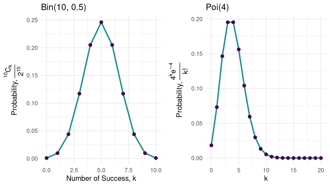 You know it’s shape is symmetric about \(x = \frac{1}{2}\) but, \(\Poi{4}\) isn’t. The shape of the distribution is governed by the nature of it’s graph around the mean, wheather it is skewed left or right.
1.2.2 Playing with Data
R contains many single valued data types to use. In this book, we will focus on three most imporatnt ones.
- Numeric Data
- Character Data surrounded by double quotes
- Logical Data
TRUEandFALSE
Vectors, Lists, Matrices
Manipulating these 4 types of data is most basic skill that will help you in data analysis. You have already seen creation and slicing of vectors. Though much of the stuffs left!
More on vectors
The functions rep(), seq() and their friends rep_len(), seq_along(), seq_len() may also help you to create vectors.
seq() creates a vector just like the colon : operator. You can spcify the gap between numbers with by = argument.
Explore the seq_along(), seq_len() functions.
The rep() function replicates the 1st argument as many times as the 2nd argument.
Lists
List is a similar to vectors but unlike vectors, it can have components with mixed data types.
Matrices
You can create this two-dimensional data structure: matrix with matrix() function specifying the entries in the 1st argument as a vector. The number of rows is spcified with nrow = and columns with ncol =. You can use both but be sure that they multiply up to match the number of entries.
mat_a <- matrix(seq(3, 5, by = 1 / 10), nrow = 7, ncol = 3)
mat_a
#>      [,1] [,2] [,3]
#> [1,]  3.0  3.7  4.4
#> [2,]  3.1  3.8  4.5
#> [3,]  3.2  3.9  4.6
#> [4,]  3.3  4.0  4.7
#> [5,]  3.4  4.1  4.8
#> [6,]  3.5  4.2  4.9
#> [7,]  3.6  4.3  5.0

## Only with number of columns
mat_b <- matrix(seq(3, 5, by = 1 / 10), ncol = 3)
It’s a good practice to specify either of the one. By default the entries filled columnwise. You may do it rowwise by setting byrow = TRUE.
The entries can be accessed with position or row number or column number.
## 4th row
mat_b[4, ]
#> [1] 3.3 4.0 4.7

## Particular entry (specifying position)
mat_a[2, 3]
#> [1] 4.5
But, you also need manipulate them. The usual entrywise operations are same as in the case of vectors: +, -, * and / (check on your own!). %*% is different, it performs matrix multiplication.
## Two matrices matching the ususal order
mat_c %*% mat_a
#>        [,1]   [,2]   [,3]
#> [1,]  76.51  92.68 108.85
#> [2,]  92.68 112.28 131.88
#> [3,] 108.85 131.88 154.91

## Matrix-vector product
mat_c %*% 1:7
#>       [,1]
#> [1,]  95.2
#> [2,] 114.8
#> [3,] 134.4
And finally, transpose can be done with t() function
t(mat_a)
#>      [,1] [,2] [,3] [,4] [,5] [,6] [,7]
#> [1,]  3.0  3.1  3.2  3.3  3.4  3.5  3.6
#> [2,]  3.7  3.8  3.9  4.0  4.1  4.2  4.3
#> [3,]  4.4  4.5  4.6  4.7  4.8  4.9  5.0
t(1:7)
#>      [,1] [,2] [,3] [,4] [,5] [,6] [,7]
#> [1,]    1    2    3    4    5    6    7
Also note that matrix can be made of strings but just like vectors if you enter mixed data types they are coerced to the same data type.
1.2.3 Dealing with data frames
A data frame is a generic data object used to store tabular data. It has three main components: the data, observations (or rows) and variables (or columns).
Create
Use the data.frame() function to create a data frame.
ka_district <- c(
  "Bagalakote", "Ballari", "Belagavi", "Bengaluru Rural", "Bengaluru Urban",
  "Bidar", "Chamarajanagara", "Chikkaballapura", "Chikkamagaluru",
  "Chitradurga", "Dakshina Kannada", " Davanagere", "Dharwada",
  "Gadag", "Hassana", "Haveri", "Kalaburagi", "Kodagu", "Kolara",
  "Koppala", "Mandya", "Mysuru", "Raichuru", "Ramanagara", "Shivamogga",
  "Tumakuru", "Udupi", "Uttara Kannada", "Vijayapura", "Yadagiri"
)

ka_dis <- c(
  215, 620, 558, 1109, 8813, 350, 780, 420,
  144, 478, 816, 242, 1051, 249, 1238, 315,
  807, 185, 1993, 515, 1997, 2886, 371, 156,
  589, 1746, 838, 964, 296, 128
)

ka_discharge <- data.frame(ka_district, ka_dis)
It is indeed a list with a specified class called data.frame!
class(ka_discharge)
#> [1] "data.frame"
mode(ka_discharge)
#> [1] "list"
sapply(ka_discharge, mode)
#> ka_district      ka_dis
#> "character"   "numeric"
But it has some restrictions4:
- all variables must be same length vectors.
data.frame(x = 1:10, y = 1:11)
#> Error in data.frame(x = 1:10, y = 1:11): arguments imply differing number of rows: 10, 11- you can’t use the same name for two different variables. R will change it.
Due to these restrictions and the resulting two-dimensional structure, data frames can mimick some of the behaviour of matrices. You can select rows and do operations on rows. You can’t do that with lists, as a row is undefined there.
You should use a data frame for any dataset that fits in that two-dimensional structure. Essentially, you use data frames for any dataset where a column coincides with a variable and a row coincides with a single observation in the broad sense of the word. For all other structures, lists are the way to go.
Note that if you want a nested structure, you have to use lists. As elements of a list can be lists themselves, you can create very flexible structured objects.
Datasets as Data frames
R consists of many builtin datasets that one can use. Run data() to list currently installed data sets.
Datasets are often stored as data frame. Let us study one example: the airquality dataset. Use help: ?airquality
Some initial stuffs
You might want to know how the data frame looks like. You can execute airquality and get it whole but datasets are large. It’s better to see some initial rows. Use head() function to print first six rows.
head(airquality)
#>   Ozone Solar.R Wind Temp Month Day
#> 1    41     190  7.4   67     5   1
#> 2    36     118  8.0   72     5   2
#> 3    12     149 12.6   74     5   3
#> 4    18     313 11.5   62     5   4
#> 5    NA      NA 14.3   56     5   5
#> 6    28      NA 14.9   66     5   6

## You may specify the number of lines
head(airquality, n = 10)
#>    Ozone Solar.R Wind Temp Month Day
#> 1     41     190  7.4   67     5   1
#> 2     36     118  8.0   72     5   2
#> 3     12     149 12.6   74     5   3
#> 4     18     313 11.5   62     5   4
#> 5     NA      NA 14.3   56     5   5
#> 6     28      NA 14.9   66     5   6
#> 7     23     299  8.6   65     5   7
#> 8     19      99 13.8   59     5   8
#> 9      8      19 20.1   61     5   9
#> 10    NA     194  8.6   69     5  10
Try the tail() function. Name is self-explanatory.
To know a specific datapoint, you can mention it’s position with numbers or the variable name and the observation number. Just like matrix!
You can get an entire observation with it’s position
airquality[148, ]
#>     Ozone Solar.R Wind Temp Month Day
#> 148    14      20 16.6   63     9  25
airquality[length(airquality$Temp), ]
#>     Ozone Solar.R Wind Temp Month Day
#> 153    20     223 11.5   68     9  30
Just like vector slicing, a data frame can be sliced with vector.
airquality[, c(1, 4)] |> head(n = 3)
#>   Ozone Temp
#> 1    41   67
#> 2    36   72
#> 3    12   74
airquality[1:3, c(1, 4)]
#>   Ozone Temp
#> 1    41   67
#> 2    36   72
#> 3    12   74
Five number summary
Five number summary is a set of descriptive statistics consisting of the five most important sample percentiles of a dataset (\(\nRV{X}{n}\)):
- the sample minimum (smallest observation) - \(X_{\left(1\right)}\)
- the lower quartile or first quartile - \(X_{\left(\left[\frac{n}{4}\right]\right)}\)
- the median (the middle value) - \(X_{\left(\left[\frac{n}{2}\right]\right)}\)
- the upper quartile or third quartile - \(X_{\left(\left[\frac{3n}{4}\right]\right)}\)
- the sample maximum (largest observation) - \(X_{\left(n\right)}\)
summary(airquality$Temp)
#>    Min. 1st Qu.  Median    Mean 3rd Qu.    Max.
#>   56.00   72.00   79.00   77.88   85.00   97.00
It gives you a rough idea about how a data set looks like.
Plotting
Histogram
par(mfrow = c(1, 2))

## left
hist(airquality$Temp)

## right: better insights
hist(airquality$Temp,
  breaks = airquality$Temp |> pretty(n = 24),
  xlab = "Temperature",
  main = "Temperature count \n New York, May-Sep 1973",
  col = "seagreen"
)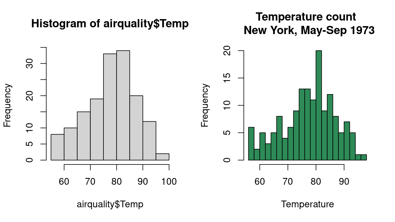
par() can be used for plotting multiple plots in a single frame, making it easy to create a figure arrangement with fine control.
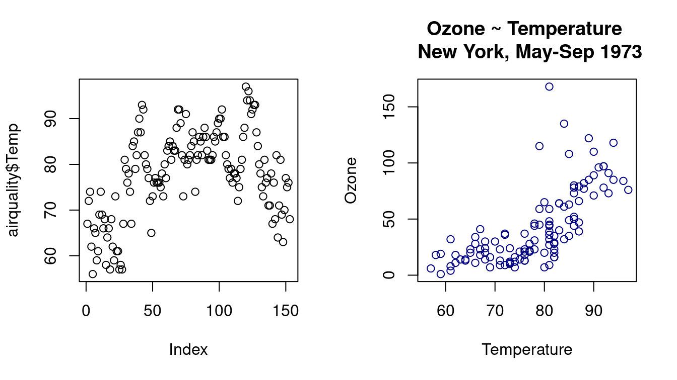
With single variable airquality$Temp, plot() function plots airquality$Temp ~ index.
par(mfrow = c(1, 2))

## left
plot(airquality$Temp)

## right: scatter plot between the mentioned variables
plot(
  y = airquality$Ozone, x = airquality$Temp,
  xlab = "Temperature", ylab = "Ozone",
  main = "Ozone ~ Temperature \n New York, May-Sep 1973",
  col = "navyblue"
)
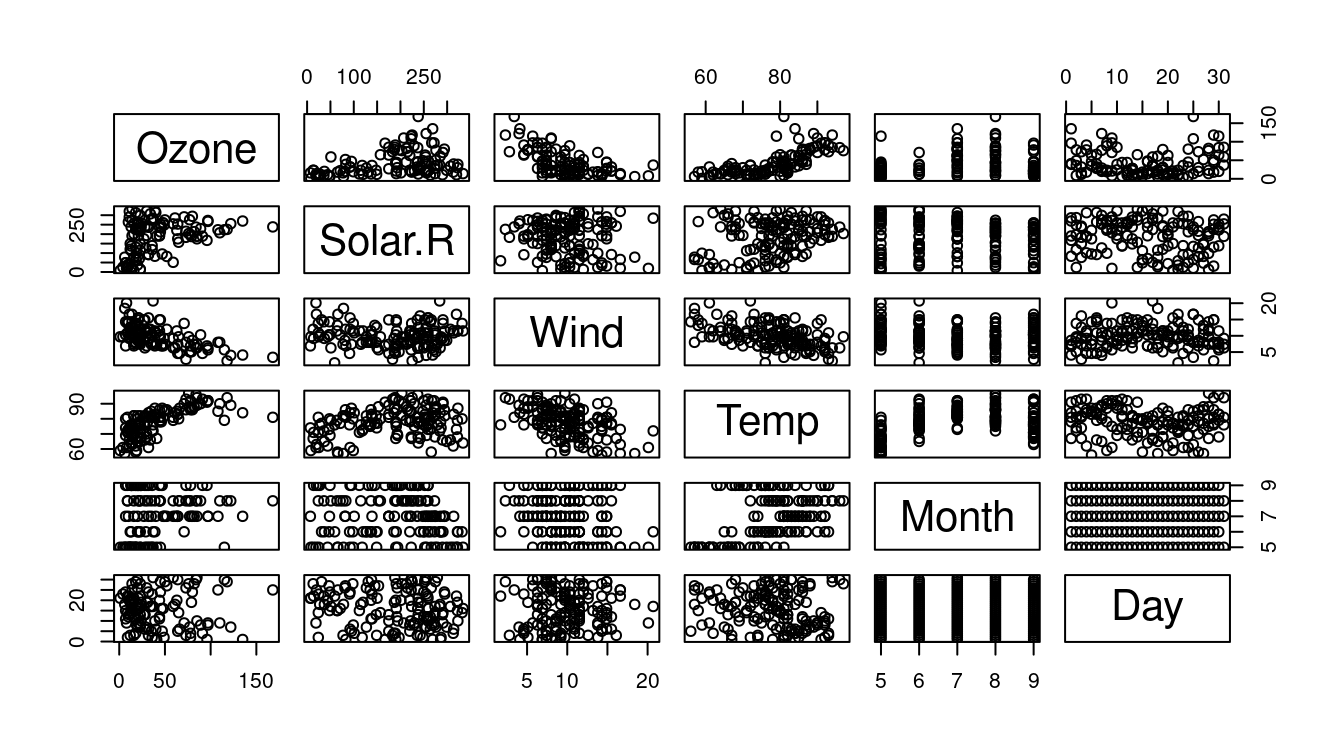
You may plot each combination of two variables just passing the whole dataset.
Reading data frames
Dataset files comes in various different formats. You can read most of them in R, inluding files created in other statistical softwares: Excel (in CSV, XLSX, or TXT format) SAS, Stata, SPSS and more.
As the name suggests read.csv() loads data from CSV (comma seperated values) formatted files and stores it into a data frame. The file = argument takes the file path and header = takes a boolean value wheather the 1st row contains the column (variable) names or not.
ka_bull_df <- read.csv(
  file = "../../assets/datasets/KAbulletin.csv",
  header = TRUE
)
class(ka_bull_df)
#> [1] "data.frame"

## column names
names(ka_bull_df)
#> [1] "District"           "Today.s.Positives"  "Total.Positives"
#> [4] "Today.s.Discharges" "Total.Discharges"   "Total.Active.Cases"
#> [7] "Today.s.Deaths"     "Deaths"
For local files, specify the file path with respect to your present workspace folder. And, if you want to load the file from an online http/https source, specify the link verbatim.
For example, you may load the above KAbulletin.csv file by downloading it or using the link: https://iscd-r.github.io/assets/datasets/KAbulletin.csv
Some other reading functions include
read.table()(white space seperated data values)read.csv2()(when data values are;seperated instead of,)read.delim()(delimited text files)read_excel()(excel files)
1.2.4 Generating random data
R contains functions to handle most of the standard probability distributions. For each of them it has four functions:
- random sample function: prefixed with
r - density function: prefixed with
d - cumulative distribution function: prefixed with
p - quantile function (aka inverse c.d.f.): prefixed with
q
Uniform random variable
Discrete
Let \(n \in \N\). \(X \sim U(\{1,2,\ldots,n\})\) is called Uniform random variable taking values in \(\{1,2,\ldots,n\}\) with probability mass function, \[\Prob{X = k} = \frac{1}{n} \ \forall \ k \in \{1,2,\ldots,n\}\]
- Rolling a fair dice 10 times
- Tossing a biased coin 10 times with success probability 0.7
Binomial random variable
Let \(n \in \N\) and \(p \in (0,1)\). \(X \sim \Bin{n,p}\) is called Binomial random variable taking values in \(\{1,2,\ldots,n\}\) with probability mass function, \[\Prob{X = k} = \binom{n}{k}p^k(1-p)^{n-k} \ \forall \ k \in \{1,2,\ldots,n\}\]
- 20 \(\Bin{6,\frac{1}{2}}\) sample
- 10 \(\Bin{30, 0.3}\) sample
See Exercise 1.8
Normal random variable
Let \(\mu \in \R, \sigma > 0\). \(X \sim N(\mu,\sigma^2)\) is called Normal random variable taking values in \(\R\) with probability mass function, \[f(x) = \frac{1}{\sqrt{2\pi}\sigma}e^{-\frac{(x-\mu)^2}{2\sigma^2}} \ \forall \ x \in \R\]
- 2 \(N(10, 25)\) sample
- 10 \(N(3, 16)\) sample
rnorm(10, mean = 3, sd = 4)
#>  [1] -2.476862  2.293486  0.842391 -0.967609  9.071873  2.637864  4.537119
#>  [8]  2.501265  2.231686  3.924981
See Exercise 1.9
Exponential random variable
Let \(\lambda > 0\). \(X \sim \Exp{\lambda}\) is said to be distributed Exponentially with parameter \(\lambda\) taking values in \(\R\) with probability mass function, \[f(x) = \begin{cases} \lambda e^{-\lambda x} &\text{ if } x > 0 \\ 0 &\text{otherwise} \end{cases} = \lambda e^{-\lambda x}\mathbb{1}\left[ x > 0 \right]\] where \(\mathbb{1}\) is the indicator function.
- 10 \(\Exp{\frac{1}{2500}}\) sample
rexp(10, 1 / 2500)
#>  [1] 3358.55756 2429.46648   45.61405 2454.83229  545.83246 1546.48566
#> [7] 1052.93050 518.34757 1375.16501 611.85440- 10 \(\Exp{3}\) sample
rexp(10, 3)
#>  [1] 0.38243272 1.91277774 0.28767228 0.46806652 0.06176535 0.13334676
#>  [7] 0.40827191 0.85497960 0.66295343 0.27423785
See Exercise 1.10
Poisson random variable
Let \(\lambda > 0\). \(X \sim \Poi{\lambda}\) is called Poisson random variable taking values in non-negetive integers with probability mass function, \[\Prob{X = k} = \frac{\lambda^k e^{-\lambda}}{k!} \ \forall \ k \in \N \cup \{0\}\]
- 10 \(\Poi{\frac{2}{5}}\) sample
- 7 \(\Poi{3}\) sample
See Exercise 1.11
1.2.5 Working With dplyr package
The Master.csv file contains Deceased data from Karnataka COVID-19 Bulletin
deceased_df <- read.csv(
  file = "../../assets/datasets/Master.csv",
  header = TRUE
)
head(deceased_df)
#>   Sno        District State.P.No Age.In.Years    Sex
#> 1   1      Kalaburagi          6           76   Male
#> 2   2 Chikkaballapura         53           70 Female
#> 3   3        Tumakuru         60           60   Male
#> 4   4      Bagalakote        125           75   Male
#> 5   5      Kalaburagi        177           65   Male
#> 6   6           Gadag        166           80 Female
#>                      Description Symptoms Co.Morbidities  DOA        DOD
#> 1 Travel history to Saudi Arabia     <NA>  HTN & Asthama <NA>       <NA>
#> 2        Travel history to Mecca     <NA>           <NA> <NA>       <NA>
#> 3        Travel history to Delhi     <NA>           <NA> <NA>       <NA>
#> 4                           <NA>     <NA>           <NA> <NA> 2020-04-03
#> 5                           SARI     <NA>           <NA> <NA>       <NA>
#> 6                           SARI     <NA>           <NA> <NA>       <NA>
#>      MB.Date Notes
#> 1 2020-03-13  <NA>
#> 2 2020-03-26  <NA>
#> 3 2020-03-27  <NA>
#> 4 2020-04-04  <NA>
#> 5 2020-04-08  <NA>
#> 6 2020-04-09  <NA>
names(deceased_df) <- c(
  "Sno", "District", "Pid", "Age", "Sex",
  "Description", "Symptoms", "CMB", "DOA",
  "DOD", "MB.Date", "Notes"
)
Some imporatnt dplyr functions:
filter():
- Extract rows that meet logical criteria
- filters data according to the given condition
Filters data by age greater than 100
filter(deceased_df, Age > 100)
#>     Sno        District     Pid Age    Sex Description
#> 1  3277 Bengaluru Urban  180841 102   Male         ILI
#> 2 17972 Bengaluru Rural 1361618 102   Male        SARI
#> 3 24686 Bengaluru Urban 1341967 102   Male        SARI
#> 4 27273 Bengaluru Urban 2360283 102 Female        SARI
#> 5 33704          Mysuru 2807010 110   Male        SARI
#> 6 34793          Haveri 2843699 101   Male       SARI
#> 7 35077           Kolar 2816836 103   Male         ILI
#> 8 37190          Kodagu 2947715 101 Female        SARI
#> 9 37373  Uttara Kannada 2996149 102   Male         ILI
#>                        Symptoms      CMB        DOA        DOD    MB.Date
#> 1                  Fever, Cough CKD, IHD 2020-08-08 2020-08-08 2020-08-10
#> 2                Breathlessness  DM, HTN 2021-04-24 2021-04-25 2021-05-08
#> 3                Breathlessness       DM 2021-04-24 2021-05-04 2021-05-23
#> 4                Breathlessness        - 2021-05-11 2021-05-25 2021-05-27
#> 5  Fever, Cough, Breathlessness        - 2021-06-12 2021-06-17 2021-06-19
#> 6 Fever, Cough, Breathlessness  DM, HTN  2021-06-18 2021-06-28 2021-06-28
#> 7                  Fever, Cough        - 2021-06-14 2021-06-30 2021-07-01
#> 8  Fever, Cough, Breathlessness        - 2021-08-01 2021-08-26 2021-08-27
#> 9                  Fever, cough      HTN       <NA> 2021-09-02 2021-09-06
#>                   Notes
#> 1                  <NA>
#> 2                  <NA>
#> 3                  <NA>
#> 4                  <NA>
#> 5                  <NA>
#> 6                  <NA>
#> 7                  <NA>
#> 8                  <NA>
#> 9 Died at his residence
Retains only the rows satisfying the given conditions
filter(deceased_df, Age > 100 & Sex == "Female")
#>     Sno        District     Pid Age    Sex Description
#> 1 27273 Bengaluru Urban 2360283 102 Female        SARI
#> 2 37190          Kodagu 2947715 101 Female        SARI
#>                       Symptoms CMB        DOA        DOD    MB.Date Notes
#> 1               Breathlessness   - 2021-05-11 2021-05-25 2021-05-27  <NA>
#> 2 Fever, Cough, Breathlessness - 2021-08-01 2021-08-26 2021-08-27 <NA>head(deceased_df$DOA)
#> [1] NA NA NA NA NA NA
head(deceased_df$MB.Date)
#> [1] "2020-03-13" "2020-03-26" "2020-03-27" "2020-04-04" "2020-04-08"
#> [6] "2020-04-09"Drop the NA rows
Can’t be done with subset()
mutate():
- To add new variable without affecting original ones
deceased_df <- mutate(
  deceased_df,
  reporting.time = as.Date(deceased_df$MB.Date) - as.Date(deceased_df$DOD)
  # Here you have added new variable "reporting.time" to the dataframe
  # Original variables are not affected
)
Similarly added a new variable Month
distinct():
- Removes rows with duplicate values
Selects distinct rows of Age variable
Other variables can be kept with .keep_all = TRUE argument
slice():
- Select rows by position
SL <- slice(deceased_df, 10:12)
head(SL, 2)
#>   Sno        District Pid Age  Sex Description       Symptoms
#> 1  24           Bidar 590  82 Male        SARI           <NA>
#> 2  25 Bengaluru Urban 557  63 Male        <NA> Breathlessness
#>                                        CMB        DOA        DOD    MB.Date
#> 1                                     <NA> 2020-04-27 2020-04-28 2020-05-02
#> 2 Diabetes & Hypertension & Hypothyroidism 2020-04-30 2020-05-02 2020-05-02
#>   Notes reporting.time Month
#> 1  <NA>         4 days   May
#> 2 <NA> 0 days Maygroup_by():
- To create a “grouped” copy of a table grouped by columns in …
dplyrfunctions will manipulate each “group” separately and combine the results.
groups data by the specified variable.
head(GS)
#> # A tibble: 6 × 14
#> # Groups:   Sex [2]
#>     Sno District          Pid   Age Sex   Description Symptoms CMB   DOA   DOD
#>   <int> <chr>           <int> <dbl> <chr> <chr>       <chr>    <chr> <chr> <chr>
#> 1     4 Bagalakote        125    75 Male  <NA>        <NA>     <NA>  <NA>  2020…
#> 2    11 Chikkaballapura   250    65 Male  <NA>        H1N1 po… DM &… 2020… 2020…
#> 3    13 Bengaluru Urban   195    66 Male  <NA>        <NA>     <NA>  2020… 2020…
#> 4    14 Vijayapura        374    42 Male  <NA>        <NA>     <NA>  2020… 2020…
#> 5    19 Bengaluru Urban   465    45 Fema… SARI        Pneumon… Daib… 2020… 2020…
#> 6    20 Kalaburagi        422    57 Male  SARI        <NA>     CLD   2020… 2020…
#> # ℹ 4 more variables: MB.Date <chr>, Notes <chr>, reporting.time <drtn>,
#> #   Month <chr>
Display does NOT show grouping, but it will specify the groups
summarise():
- Compute table of summaries
- Summarises multiple values into a single value
Gives the mean of age for each gender.
sample_n():
- To select random rows according to the value specified
Selects 2 random rows from dataframe deceased_df.
sample_n(deceased_df, size = 2)
#>     Sno        District     Pid Age  Sex Description              Symptoms
#> 1 26593 Bengaluru Urban 1839041  75 Male        SARI Fever, Breathlessness
#> 2  9105 Bengaluru Urban  600977  65 Male        SARI        Breathlessness
#>        CMB        DOA        DOD    MB.Date                 Notes
#> 1 HTN, IHD       <NA> 2021-05-09 2021-05-26 Died at his residence
#> 2      IHD 2020-09-29 2020-09-29 2020-10-02                  <NA>
#>   reporting.time   Month
#> 1        17 days     May
#> 2         3 days October
Selects 0.0001-fraction of rows at random.
sample_frac(deceased_df, size = 0.0001)
#>     Sno        District     Pid Age    Sex Description
#> 1 31188 Bengaluru Urban 2629021  85 Female         ILI
#> 2 19862 Bengaluru Urban 1192493  79 Female        SARI
#> 3  1874 Bengaluru Urban   50930  80   Male         ILI
#> 4 35683 Bengaluru Urban 2867489  66 Female        SARI
#>                       Symptoms     CMB        DOA        DOD    MB.Date Notes
#> 1                 Fever, Cough DM, HTN 2021-05-29 2021-06-04 2021-06-05  <NA>
#> 2 Fever, Cough, Breathlessness DM, HTN 2021-04-18 2021-05-08 2021-05-12  <NA>
#> 3               Breathlessness     HTN 2020-07-18 2020-07-18 2020-07-27  <NA>
#> 4        Fever, Breathlessness     HTN 2021-06-24 2021-07-08 2021-07-09  <NA>
#>   reporting.time Month
#> 1         1 days  June
#> 2         4 days   May
#> 3         9 days  July
#> 4 1 days Julyarrange():
- Order rows by values of a column or columns (low to high)
- use with desc() to order from high to low
Creates a new dataframe orderdf having rows arranged by - Age.
head(orderdf, 2)
#>     Sno        District     Pid    Age    Sex Description       Symptoms CMB
#> 1 14253 Bengaluru Urban 1260623 0.0000   Male        SARI Breathlessness HTN
#> 2 20970      Ramanagara 2032210 0.0082 Female        SARI Breathlessness   -
#>          DOA        DOD    MB.Date Notes reporting.time Month
#> 1 2021-04-21 2021-04-23 2021-04-24  <NA>         1 days April
#> 2 2021-05-07 2021-05-10 2021-05-14  <NA>         4 days   May
Arranges the data in alphabetical order of the variable - Description
1.2.5.1 The pipe operator - %>%
- Used to chain codes
x %>% f(y)becomesf(x, y)
filtered_data <- filter(deceased_df, Month != "September")
grouped_data <- group_by(filtered_data, Month)
summarise(grouped_data, mean(Age, na.rm = TRUE))
#> # A tibble: 11 × 2
#>   Month    `mean(Age, na.rm = TRUE)`
#>   <chr>                        <dbl>
#> 1 April                         61.2
#> 2 August                        61.3
#> 3 December                      64.9
#> 4 February                      65.3
#> 5 January                       63.6
#> 6 July                          60.0
#> # ℹ 5 more rows
The same code written shortly with Pipe - %>%
Exercises
Exercise 1.4 (Dice Experiment) Rolling a die 1500 Times.
x <- c(1, 2, 3, 4, 5, 6)
prob_x <- c(1 / 8, 1 / 8, 1 / 8, 1 / 8, 3 / 8, 1 / 8)
f_1500 <- sample(x, size = 1500, replace = TRUE, prob = prob_x)- Describe what each R statement is performing in the above.
- Using the
mean()andvar()function find the mean and variance off_1500. From this information alone what would you conclude is the range of the random variablef_1500. - Does the mean and variance from the sample generated compare closely with the true mean and variance of
f_1500.
Exercise 1.5 (Sums of Rolls) Suppose you wish to simulate in R the experiment of Rolling a die 5 times and noting down its sum. You can use the sample(), matrix() and apply() functions.
x <- c(1, 2, 3, 4, 5, 6)
prob_x <- c(1 / 6, 1 / 6, 1 / 6, 1 / 6, 1 / 6, 1 / 6)
rolls <- sample(x, size = 1500, replace = TRUE, prob = prob_x)
rolls_mat <- matrix(rolls, nrow = 5)
roll_sums <- apply(rolls_mat, 2, sum)- Describe the functions
matrix()andapply() - Run the following R-code and observe the picture. What does \(\displaystyle\int_{12}^{21}\)
norm_density(\(x,\mu,\sigma\))\(\dd{x}\) approximate?
library("ggplot2")
norm_density <- function(x, a, s) {
  (1 / ((2 * pi)^(0.5) * s)) * exp(-(x - a)^2 / (2 * s^2))
}

df_rolls <- data.frame(roll_sums)
mu <- mean(df_rolls$roll_sums)
sigma <- sd(df_rolls$roll_sums)

ggplot(data = df_rolls) +
  geom_histogram(
    mapping = aes(x = roll_sums, y = ..density..),
    color = "#00846b",
    fill = NA,
    binwidth = 1
  ) +
  xlim(5, 30) +
  geom_function(
    fun = norm_density,
    args = list(a = mu, s = sigma),
    color = "black"
)- If \[\begin{align} \text{Area under the histogram between 12 and 21 } \approx \int_{a}^{b} \frac{1}{\sqrt{2\pi}}\exp\left( -\frac{x^2}{2} \right)\dd{x} \end{align}\] then what would be your guess for \(a\) and \(b\)?
Exercise 1.6 Use the dplyr package to do the following computations.
- Create a new data frame
iris_1that contains only the speciesvirginicaandversicolorwith sepal lengths longer than 6cm and sepal widths longer than 2.5cm. How many observations and variables are in the dataset? - Now, create a
iris_2data frame fromiris_1that contains only the columns forSpecies,Sepal.Length, andSepal.Width. How many observations and variables are in the dataset? - Create an
iris_3data frame fromiris_2that orders the observations from largest to smallest sepal length. Show the first 6 rows of this dataset. - Create an
iris_4data frame fromiris_3that creates a column with aSepal.Area(length \(\X\) width) value for each observation. How many observations and variables are in the dataset? - Create
iris_5that calculates the average sepal length, the average sepal width, and the sample size of the entireiris_4data frame and printiris_5. - Finally, create
iris_6that calculates the average sepal length, the average sepal width, and the sample size for each species of in theiris_4data frame and printiris_6. - In these exercises, you have successively modified different versions of the data frame
iris_1,iris_2,iris_3,iris_4,iris_5,iris_6. At each stage, the output data frame from one operation serves as the input fro the next. A more easy way to do this is to use the pipe operator%>%from thetidyrpackage. Rework all of your previous statements into an extended piping operation that usesirisas the input and generatesiris_6as the output.
Exercise 1.7 (Coin Toss Experiment) Do the following:
- Tossing a coin 10 times.
- Using the
?rbinomexplain what each of the above functions is performing in R. - Using the
mean()andvar()function find the mean and variance ofbin_1,bin_2,bin_3. Compare them with the true mean and variance of the respective Binomial distribution.
geom_hist()function.
library(ggplot2)
df_bin_1 <- data.frame(bin_1)
plt_1_1 <- ggplot(df_bin_1) +
  geom_histogram(
    mapping = aes(x = bin_1),
    color = "#00846b",
    fill = "NA",
    binwidth = 1
  )
plt_2_1 <- ggplot(df_bin_1) +
  geom_histogram(
    mapping = aes(x = bin_1, y = ..density..),
    color = "#00846b",
    fill = "NA",
    binwidth = 1
)- Explain what are the plots
plt_1_1,plt_2_1providing. - Rewrite the code to provide the plots for
bin_2andbin_3. - What can you say about the three plots?
- (Density Approximation) The below code plots the
norm_density()function in the interval \([0, 10]\) witha\(= 5\),s\(= \sqrt{2.5}\) along with the plotplt_2_1.
library("ggplot2")

norm_density <- function(x, a, s) {
  (1 / ((2 * pi)^(0.5) * s)) * exp(-(x - a)^2 / (2 * s^2))
}
df_bin_1 <- data.frame(bin_1)

ggplot(df_bin_1) +
  geom_histogram(
    mapping = aes(x = bin_1, y = ..density..),
    color = "#00846b", fill = "NA", binwidth = 1
  ) +
  xlim(0, 10) +
geom_function(fun = norm_density, args = list(a = 5, s = (2.5)^(0.5)))- From the picture what does \(\displaystyle\int_{3}^{6}\)
norm_density(\(x,\mu,\sigma\))\(\dd{x}\) approximate? - If \[\begin{align} \text{Area under the histogram between 3 and 7 } \approx \int_{c}^{d} \frac{1}{\sqrt{2\pi}}\exp\left( -\frac{x^2}{2} \right)\dd{x} \end{align}\] then what would be your guess for \(c\) and \(d\)?
- How would you try the same idea for
bin_2andbin_3? Would you get the same result?
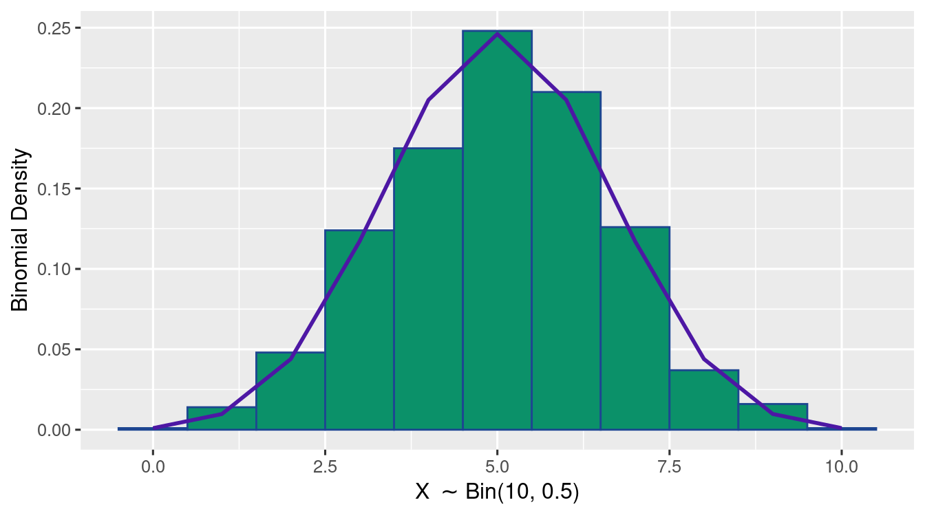
Exercise 1.8 (Binomial Distribution Plot) Generate 1000 samples of \(\Bin{10,0.5}\). Using ggplot(), write R-code to plot a histogram of relative frequency along with a lineplot of the true Binomial probabilities.
(as shown in the figure)
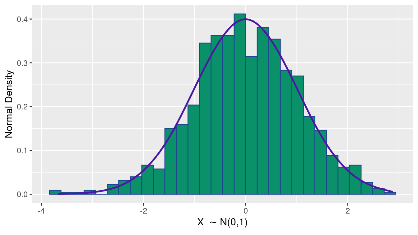
Exercise 1.9 (Normal Distribution Plot) Generate 1000 samples of \(N(0,1)\). Using ggplot(), write R-code to plot a histogram of relative frequency along with a lineplot of the true Normal probabilities.
(as shown in the figure)
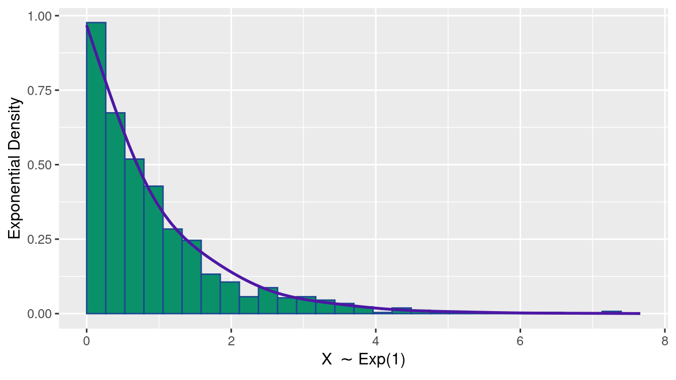
Exercise 1.10 (Exponential Distribution Plot) Generate 1000 samples of \(\Exp{1}\). Using ggplot(), write R-code to plot a histogram of relative frequency along with a lineplot of the true Exponential probabilities.
(as shown in the figure)
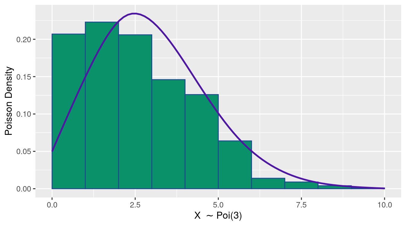
Exercise 1.11 (Poisson Distribution Plot) Generate 1000 samples of \(\Poi{3}\). Using ggplot(), write R-code to plot a histogram of relative frequency along with a lineplot of the true Poisson probabilities.
(as shown in the figure)