\[ \newcommand{\nRV}[2]{{#1}_1, {#1}_2, \ldots, {#1}_{#2}} \newcommand{\pnRV}[3]{{#1}_1^{#3}, {#1}_2^{#3}, \ldots, {#1}_{#2}^{#3}} \newcommand{\onRV}[2]{{#1}_{(1)} \le {#1}_{(2)} \le \ldots \le {#1}_{(#2)}} \newcommand{\RR}{\mathbb{R}} \newcommand{\Prob}[1]{\mathbb{P}\left({#1}\right)} \newcommand{\PP}{\mathcal{P}} \newcommand{\iidd}{\overset{\mathsf{iid}}{\sim}} \newcommand{\X}{\times} \newcommand{\EE}[1]{\mathbb{E}\left[{#1}\right]} \newcommand{\Var}[1]{\mathsf{Var}\left({#1}\right)} \newcommand{\Ber}[1]{\mathsf{Ber}\left({#1}\right)} \newcommand{\Geom}[1]{\mathsf{Geom}\left({#1}\right)} \newcommand{\Bin}[1]{\mathsf{Bin}\left({#1}\right)} \newcommand{\Poi}[1]{\mathsf{Pois}\left({#1}\right)} \newcommand{\Exp}[1]{\mathsf{Exp}\left({#1}\right)} \newcommand{\SD}[1]{\mathsf{SD}\left({#1}\right)} \newcommand{\sgn}[1]{\mathsf{sgn}} \newcommand{\dd}[1]{\operatorname{d}\!{#1}} \]

3.4 Examining Normality

Suppose \(X \sim N(\mu,\sigma^2)\) then \(X\) has pdf given by, \[\begin{align*} f(x) = \frac{e^{-\frac{(x-\mu)^2}{2\sigma^2}}}{\sqrt{2\pi}\sigma}, x \in \RR \end{align*}\] and cdf of \(X\), \[\begin{align*} F(x) = \Prob{X \leq x} = \int_{-\infty}^{x} f(t)\dd{t} = \int_{-\infty}^{x} \frac{e^{-\frac{(t-\mu)^2}{2\sigma^2}}}{\sqrt{2\pi}\sigma} \dd{t} \end{align*}\] But this integral can’t be evaluated explicitely. So, the values are computed numerically. They are listed in Normal tables (also known as \(Z-\)tables). In R, pnorm(q = a) function returns the value of \(F(\)a\()\).

pnorm(q = 0)
#> [1] 0.5
pnorm(q = 0, lower.tail = TRUE)
#> [1] 0.5

Normal distribution

Observations for checking normality in data

\(68-95-99\) rule

\[\begin{align*} &\Prob{\left| X-\mu \right| < \sigma} &= \int_{\mu-\sigma}^{\mu+\sigma}f(x)\dd{x} &\approx 0.68 \\ &\Prob{\left| X-\mu \right| < 2\sigma} &= \int_{\mu-2\sigma}^{\mu+2\sigma}f(x)\dd{x} &\approx 0.95 \\ &\Prob{\left| X-\mu \right| < 3\sigma} &= \int_{\mu-3\sigma}^{\mu+3\sigma}f(x)\dd{x} &\approx 0.99 \end{align*}\]

Skewness & Kurtosis

\[\begin{equation} \tag{3.10} \textsf{Skewness} = \sum_{i=1}^{n} \left(\frac{X_i-\overline{X}}{\sigma_X}\right)^3 \end{equation}\] \[\begin{equation} \tag{3.11} \textsf{Kurtosis} = \sum_{i=1}^{n} \left(\frac{X_i-\overline{X}}{\sigma_X}\right)^4 \end{equation}\]

• Skewness measures the lack of symmetry in the distribution. If \(\textsf{Skewness} = 0\) then the distribution is symmetric.
• \(\textsf{Kurtosis}\) (though harder to inerpret) measures the peakedness or flatness of the distribution.

If data \(X_1, X_2, \dots, X_n\) has \(\textsf{Skewness}\) “far” from \(0\) and \(\textsf{Kurtosis}\) “far” from \(3\) then we conclude that, Data is not normal.

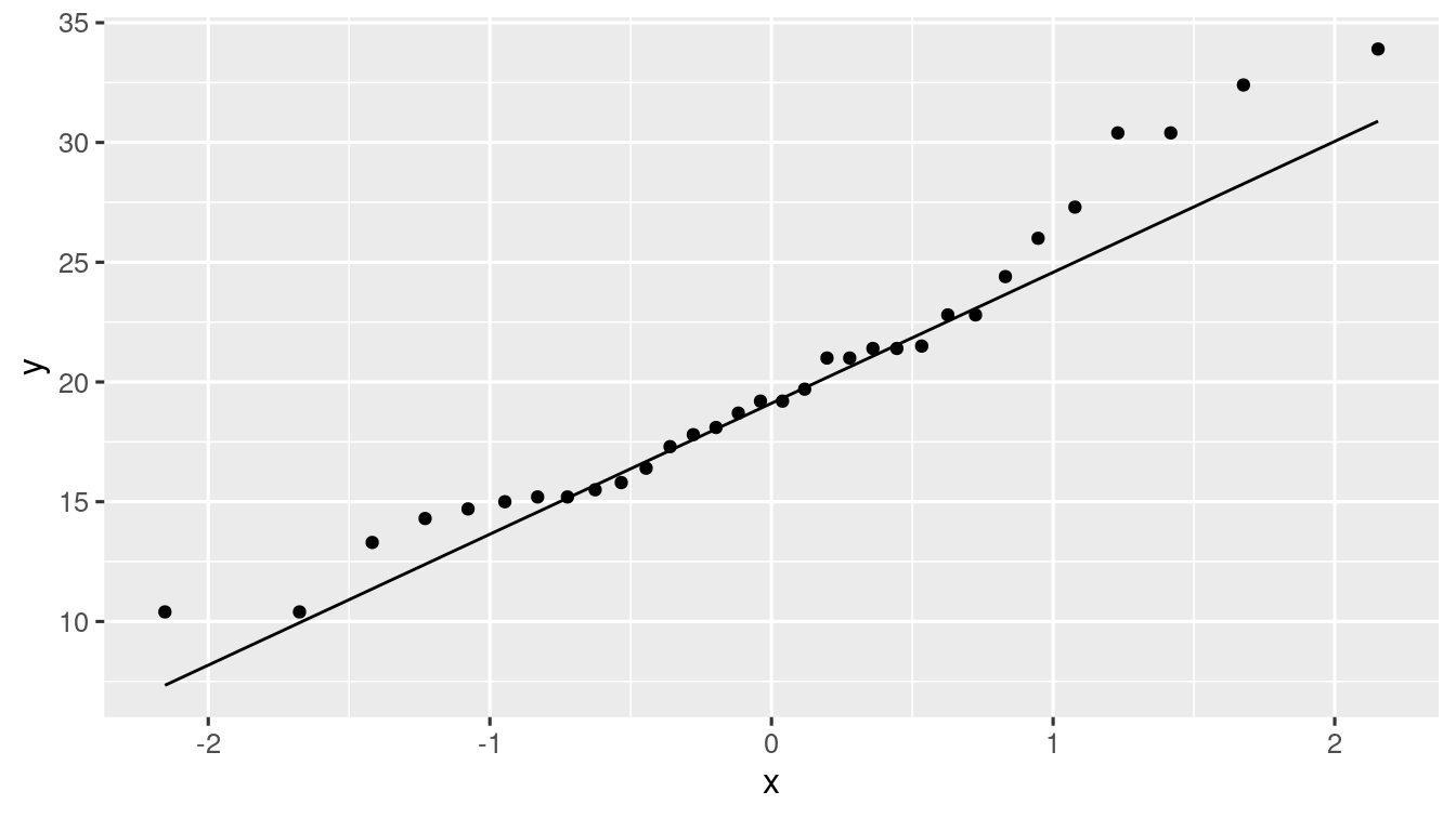
Q-Q plot

Consder the data \({\bf X} = (X_1, X_2, \dots, X_n)\). \(\onRV{X}{n}\) be the order statistic. Call \(X_{(k)}\) to be the \(\frac{k}{n+1} -\)sample quantile.

For, \(\alpha \in (0,1)\) find \(z_{\alpha}\) such that \[ \Prob{X \leq z_{\alpha}} = \alpha (= \alpha^\textsf{th}-\textsf{quantile of Normal}) \] Then, plotting \(\left\{ \left( z_\frac{k}{n+1},X_{k} \right) : k = 0,1,\ldots,n \right\}\) we will obtain the Q-Q plot for the data.
If plot is not a straight line then the Data is most likely not normal.

In R, you can get Q-Q plot with geom_qq() function.

ggplot(mtcars, aes(sample = mpg)) +
  geom_qq() +
  geom_qq_line()

Exercises

Exercise 3.10 Write an R-code to perform the following:

1. Using replicate() generate \(100\) realisations of \(Y\) and \(Z\) as described below:
   1. Generate 15 samples from \(\Poi{10}\) distribution
   2. Compute the sample mean \(\overline{X}\) and sample variance \(S^2\) of the generated sample.
   3. Compute \(Y = \sqrt{15}\left( \frac{\overline{X} - \mu}{\sigma} \right)\), where \(\mu\) and \(\sigma\) are the mean and variance of the \(\Poi{10}\) distribution.
   4. Compute \(Z = \sqrt{15}\left( \frac{\overline{X} - \mu}{S} \right)\) where \(\mu\) is the mean of the \(\Poi{10}\) distribution.
2. Using Q-Q plot decide if \(Y\) or \(Z\) is Normally distributed.